Introduction

In previous presentations, we [AR, AvM] talked about stochastic differential equations (middle box in Fig. 1). Examples:

Brownian motion

$\dot{X}(t)=\xi (t)$

$X(t)=\mathcal{N}(0,t)$

Brownian motion

$\dot{X}(t)=\xi (t)$

$X(t)=\mathcal{N}(0,t)$

Drift-diffusion processes

$\dot{X}(t)=f(t,X)+\xi (t)$

$dX(t)=f(t,X)dt+g(t,X)dW$

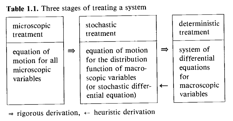
Fig. 1 (Risken, Table 1.1)

We also talked about the fact that the “white noise” $\xi$ in a Langevin equation is ill-defined.

Note

All of these conventions are defined in terms of finite intervals.

Itô convention

$$\Delta X(t_i)=f(t_i,X(t_i))\Delta t+g(t_i,X(t_i))\Delta W(t_i))\phantom{+g(t_{i+1},X(t_{i+1}))}$$

Stratonovich convention

$$\Delta X(t_i)=f(t_i,X(t_i))\Delta t+\frac{g(t_i,X(t_i))+g(t_{i+1},X(t_{i+1}))}{2}\Delta W(t_i)$$

Anticipatory (or Hänggi-Klimontovich) convention

$$\Delta X(t_i)=f(t_i,X(t_i))\Delta t+g(t_{i+1},X(t_{i+1}))\Delta W(t_i)\phantom{+g(t_i,X)}$$

This ambiguity of convention arises because the infinitesimal limit of white noise is mathematically well-defined (within a given convention), but non physical.

A full solution to a Langevin equation typically takes the form of a probability density function (PDF), which, if the system is Markovian, can be written as $p(t,X)$. Now, this PDF is physical, so a differential equation for $p(t,X)$ should not suffer from ambiguity. The Fokker-Planck equation is such a differential equation:

(1)$$\frac{\partial p(t,x)}{\partial t}=-\sum _i\frac{\partial }{\partial x_i}[D_i^{(1)}(x)p(t,x)]+\sum _{i,j}\frac{{\partial }^2}{\partial x_i\partial x_j}[D_{ij}^{(2)}(x)p(t,x)]$$

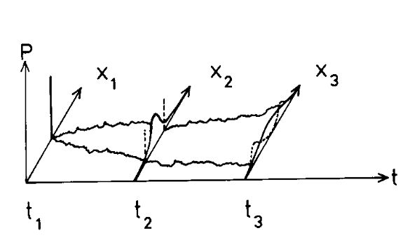
Fig. 2 The kind of problem we want to solve: given an initial probability distribution, how does it evolve over time ? Often, but not always, the initial condition is a Dirac δ. (Risken, Fig. 2.2)

A stochastic process is a generalization of a random variable. Intuitively, we assign to each $t\in \mathbb{R}$ a random variable (as suggested by Fig. 2). More precisely, to any countable set of times, the process associates a joint distribution. So if $x\in {\mathbb{R}}^{\mathbb{N}}$,

• $p(t_1,x_1)$ is the PDF of a random variable on ${\mathbb{R}}^N$;

• $p(t_2,x_2,t_1,x_1)$ is the PDF of a random variable on ${\mathbb{R}}^{2N}$;

• $p(t_3,x_3,t_2,x_2,t_1,x_1)$ is the PDF of a random variable on ${\mathbb{R}}^{3N}$;

• etc.

One obtains a lower dimensional distribution by marginalising over certain time points:

$$p(t_3,x_3,t_1,x_1)=\int p(t_3,x_3,t_2,x_2,t_1,x_1)d{x}_2$$

Markov process: $p(t_3,x_3\mid t_2,x_2,t_1,x_1)=p(t_3,x_3\mid t_2,x_2)$

For a Markov process, this becomes the Chapman-Kolmogorov equation:

$$p(t_3,x_3\mid t_1,x_1)=\int p(t_3,x_3\mid t_2,x_2)p(t_2,x_2\mid t_1,x_1)$$