Code for comparing models of the pyloric circuit#
\(\require{mathtools} \newcommand{\notag}{} \newcommand{\tag}{} \newcommand{\label}[1]{} \newcommand{\sfrac}[2]{#1/#2} \newcommand{\bm}[1]{\boldsymbol{#1}} \newcommand{\num}[1]{#1} \newcommand{\qty}[2]{#1\,#2} \renewenvironment{align} {\begin{aligned}} {\end{aligned}} \renewenvironment{alignat} {\begin{alignedat}} {\end{alignedat}} \newcommand{\pdfmspace}[1]{} % Ignore PDF-only spacing commands \newcommand{\htmlmspace}[1]{\mspace{#1}} % Ignore PDF-only spacing commands \newcommand{\scaleto}[2]{#1} % Allow to use scaleto from scalerel package \newcommand{\RR}{\mathbb R} \newcommand{\NN}{\mathbb N} \newcommand{\PP}{\mathbb P} \newcommand{\EE}{\mathbb E} \newcommand{\XX}{\mathbb X} \newcommand{\ZZ}{\mathbb Z} \newcommand{\QQ}{\mathbb Q} \newcommand{\fF}{\mathcal F} \newcommand{\dD}{\mathcal D} \newcommand{\lL}{\mathcal L} \newcommand{\gG}{\mathcal G} \newcommand{\hH}{\mathcal H} \newcommand{\nN}{\mathcal N} \newcommand{\pP}{\mathcal P} \newcommand{\BB}{\mathbb B} \newcommand{\Exp}{\operatorname{Exp}} \newcommand{\Binomial}{\operatorname{Binomial}} \newcommand{\Poisson}{\operatorname{Poisson}} \newcommand{\linop}{\mathcal{L}(\mathbb{B})} \newcommand{\linopell}{\mathcal{L}(\ell_1)} \DeclareMathOperator{\trace}{trace} \DeclareMathOperator{\Var}{Var} \DeclareMathOperator{\Span}{span} \DeclareMathOperator{\proj}{proj} \DeclareMathOperator{\col}{col} \DeclareMathOperator*{\argmin}{arg\,min} \DeclareMathOperator*{\argmax}{arg\,max} \DeclareMathOperator*{\gt}{>} \definecolor{highlight-blue}{RGB}{0,123,255} % definition, theorem, proposition \definecolor{highlight-yellow}{RGB}{255,193,7} % lemma, conjecture, example \definecolor{highlight-orange}{RGB}{253,126,20} % criterion, corollary, property \definecolor{highlight-red}{RGB}{220,53,69} % criterion \newcommand{\logL}{\ell} \newcommand{\eE}{\mathcal{E}} \newcommand{\oO}{\mathcal{O}} \newcommand{\defeq}{\stackrel{\mathrm{def}}{=}} \newcommand{\Bspec}{\mathcal{B}} % Spectral radiance \newcommand{\X}{\mathcal{X}} % X space \newcommand{\Y}{\mathcal{Y}} % Y space \newcommand{\M}{\mathcal{M}} % Model \newcommand{\Tspace}{\mathcal{T}} \newcommand{\Vspace}{\mathcal{V}} \newcommand{\Mtrue}{\mathcal{M}_{\mathrm{true}}} \newcommand{\MP}{\M_{\mathrm{P}}} \newcommand{\MRJ}{\M_{\mathrm{RJ}}} \newcommand{\qproc}{\mathfrak{Q}} \newcommand{\D}{\mathcal{D}} % Data (true or generic) \newcommand{\Dt}{\tilde{\mathcal{D}}} \newcommand{\Phit}{\widetilde{\Phi}} \newcommand{\Phis}{\Phi^*} \newcommand{\qt}{\tilde{q}} \newcommand{\qs}{q^*} \newcommand{\qh}{\hat{q}} \newcommand{\AB}[1]{\mathtt{AB}~\mathtt{#1}} \newcommand{\LP}[1]{\mathtt{LP}~\mathtt{#1}} \newcommand{\NML}{\mathrm{NML}} \newcommand{\iI}{\mathcal{I}} \newcommand{\true}{\mathrm{true}} \newcommand{\dist}{D} \newcommand{\Mtheo}[1]{\mathcal{M}_{#1}} % Model (theoretical model); index: param set \newcommand{\DL}[1][L]{\mathcal{D}^{(#1)}} % Data (RV or generic) \newcommand{\DLp}[1][L]{\mathcal{D}^{(#1')}} % Data (RV or generic) \newcommand{\DtL}[1][L]{\tilde{\mathcal{D}}^{(#1)}} % Data (RV or generic) \newcommand{\DpL}[1][L]{{\mathcal{D}'}^{(#1)}} % Data (RV or generic) \newcommand{\Dobs}[1][]{\mathcal{D}_{\mathrm{obs}}^{#1}} % Data (observed) \newcommand{\calibset}{\mathcal{C}} \newcommand{\N}{\mathcal{N}} % Normal distribution \newcommand{\Z}{\mathcal{Z}} % Partition function \newcommand{\VV}{\mathbb{V}} % Variance \newcommand{\T}{\mathsf{T}} % Transpose \newcommand{\EMD}{\mathrm{EMD}} \newcommand{\dEMD}{d_{\mathrm{EMD}}} \newcommand{\dEMDtilde}{\tilde{d}_{\mathrm{EMD}}} \newcommand{\dEMDsafe}{d_{\mathrm{EMD}}^{\text{(safe)}}} \newcommand{\e}{ε} % Model confusion threshold \newcommand{\falsifythreshold}{ε} \newcommand{\bayes}[1][]{B_{#1}} \newcommand{\bayesthresh}[1][]{B_{0}} \newcommand{\bayesm}[1][]{B^{\mathcal{M}}_{#1}} \newcommand{\bayesl}[1][]{B^l_{#1}} \newcommand{\bayesphys}[1][]{B^{{p}}_{#1}} \newcommand{\Bconf}[1]{B^{\mathrm{epis}}_{#1}} \newcommand{\Bemd}[1]{B^{\mathrm{EMD}}_{#1}} \newcommand{\BQ}[1]{B^{Q}_{#1}} \newcommand{\Bconfbin}[1][]{\bar{B}^{\mathrm{conf}}_{#1}} \newcommand{\Bemdbin}[1][]{\bar{B}_{#1}^{\mathrm{EMD}}} \newcommand{\bin}{\mathcal{B}} \newcommand{\Bconft}[1][]{\tilde{B}^{\mathrm{conf}}_{#1}} \newcommand{\fc}{f_c} \newcommand{\fcbin}{\bar{f}_c} \newcommand{\paramphys}[1][]{Θ^{{p}}_{#1}} \newcommand{\paramobs}[1][]{Θ^{ε}_{#1}} \newcommand{\test}{\mathrm{test}} \newcommand{\train}{\mathrm{train}} \newcommand{\synth}{\mathrm{synth}} \newcommand{\rep}{\mathrm{rep}} \newcommand{\MNtrue}{\mathcal{M}^{{p}}_{\text{true}}} \newcommand{\MN}[1][]{\mathcal{M}^{{p}}_{#1}} \newcommand{\MNA}{\mathcal{M}^{{p}}_{Θ_A}} \newcommand{\MNB}{\mathcal{M}^{{p}}_{Θ_B}} \newcommand{\Me}[1][]{\mathcal{M}^ε_{#1}} \newcommand{\Metrue}{\mathcal{M}^ε_{\text{true}}} \newcommand{\Meobs}{\mathcal{M}^ε_{\text{obs}}} \newcommand{\Meh}[1][]{\hat{\mathcal{M}}^ε_{#1}} \newcommand{\MNa}{\mathcal{M}^{\mathcal{N}}_a} \newcommand{\MeA}{\mathcal{M}^ε_A} \newcommand{\MeB}{\mathcal{M}^ε_B} \newcommand{\Ms}{\mathcal{M}^*} \newcommand{\MsA}{\mathcal{M}^*_A} \newcommand{\MsB}{\mathcal{M}^*_B} \newcommand{\Msa}{\mathcal{M}^*_a} \newcommand{\MsAz}{\mathcal{M}^*_{A,z}} \newcommand{\MsBz}{\mathcal{M}^*_{B,z}} \newcommand{\Msaz}{\mathcal{M}^*_{a,z}} \newcommand{\MeAz}{\mathcal{M}^ε_{A,z}} \newcommand{\MeBz}{\mathcal{M}^ε_{B,z}} \newcommand{\Meaz}{\mathcal{M}^ε_{a,z}} \newcommand{\zo}{z^{0}} \renewcommand{\lL}[2][]{\mathcal{L}_{#1|{#2}}} % likelihood \newcommand{\Lavg}[2][]{\mathcal{L}^{/#2}_{#1}} % Geometric average of likelihood \newcommand{\lLphys}[2][]{\mathcal{L}^{{p}}_{#1|#2}} \newcommand{\Lavgphys}[2][]{\mathcal{L}^{{p}/#2}_{#1}} % Geometric average of likelihood \newcommand{\lLL}[3][]{\mathcal{L}^{(#3)}_{#1|#2}} \newcommand{\lLphysL}[3][]{\mathcal{L}^{{p},(#3)}_{#1|#2}} \newcommand{\lnL}[2][]{l_{#1|#2}} % Per-sample log likelihood \newcommand{\lnLt}[2][]{\widetilde{l}_{#1|#2}} \newcommand{\lnLtt}{\widetilde{l}} % Used only in path_sampling \newcommand{\lnLh}[1][]{\hat{l}_{#1}} \newcommand{\lnLphys}[2][]{l^{{p}}_{#1|#2}} \newcommand{\lnLphysL}[3][]{l^{{p},(#3)}_{#1|#2}} \newcommand{\Elmu}[2][1]{μ_{{#2}}^{(#1)}} \newcommand{\Elmuh}[2][1]{\hat{μ}_{{#2}}^{(#1)}} \newcommand{\Elsig}[2][1]{Σ_{{#2}}^{(#1)}} \newcommand{\Elsigh}[2][1]{\hat{Σ}_{{#2}}^{(#1)}} \newcommand{\pathP}{\mathop{{p}}} % Path-sampling process (generic) \newcommand{\pathPhb}{\mathop{{p}}_{\mathrm{Beta}}} % Path-sampling process (hierarchical beta) \newcommand{\interval}{\mathcal{I}} \newcommand{\Phiset}[1]{\{\Phi\}^{\small (#1)}} \newcommand{\Phipart}[1]{\{\mathcal{I}_Φ\}^{\small (#1)}} \newcommand{\qhset}[1]{\{\qh\}^{\small (#1)}} \newcommand{\Dqpart}[1]{\{Δ\qh_{2^{#1}}\}} \newcommand{\LsAzl}{\mathcal{L}_{\smash{{}^{\,*}_A},z,L}} \newcommand{\LsBzl}{\mathcal{L}_{\smash{{}^{\,*}_B},z,L}} \newcommand{\lsA}{l_{\smash{{}^{\,*}_A}}} \newcommand{\lsB}{l_{\smash{{}^{\,*}_B}}} \newcommand{\lsAz}{l_{\smash{{}^{\,*}_A},z}} \newcommand{\lsAzj}{l_{\smash{{}^{\,*}_A},z_j}} \newcommand{\lsAzo}{l_{\smash{{}^{\,*}_A},z^0}} \newcommand{\leAz}{l_{\smash{{}^{\,ε}_A},z}} \newcommand{\lsAez}{l_{\smash{{}^{*ε}_A},z}} \newcommand{\lsBz}{l_{\smash{{}^{\,*}_B},z}} \newcommand{\lsBzj}{l_{\smash{{}^{\,*}_B},z_j}} \newcommand{\lsBzo}{l_{\smash{{}^{\,*}_B},z^0}} \newcommand{\leBz}{l_{\smash{{}^{\,ε}_B},z}} \newcommand{\lsBez}{l_{\smash{{}^{*ε}_B},z}} \newcommand{\LaszL}{\mathcal{L}_{\smash{{}^{*}_a},z,L}} \newcommand{\lasz}{l_{\smash{{}^{*}_a},z}} \newcommand{\laszj}{l_{\smash{{}^{*}_a},z_j}} \newcommand{\laszo}{l_{\smash{{}^{*}_a},z^0}} \newcommand{\laez}{l_{\smash{{}^{ε}_a},z}} \newcommand{\lasez}{l_{\smash{{}^{*ε}_a},z}} \newcommand{\lhatasz}{\hat{l}_{\smash{{}^{*}_a},z}} \newcommand{\pasz}{p_{\smash{{}^{*}_a},z}} \newcommand{\paez}{p_{\smash{{}^{ε}_a},z}} \newcommand{\pasez}{p_{\smash{{}^{*ε}_a},z}} \newcommand{\phatsaz}{\hat{p}_{\smash{{}^{*}_a},z}} \newcommand{\phateaz}{\hat{p}_{\smash{{}^{ε}_a},z}} \newcommand{\phatseaz}{\hat{p}_{\smash{{}^{*ε}_a},z}} \newcommand{\Phil}[2][]{Φ_{#1|#2}} % Φ_{\la} \newcommand{\Philt}[2][]{\widetilde{Φ}_{#1|#2}} % Φ_{\la} \newcommand{\Philhat}[2][]{\hat{Φ}_{#1|#2}} % Φ_{\la} \newcommand{\Philsaz}{Φ_{\smash{{}^{*}_a},z}} % Φ_{\lasz} \newcommand{\Phileaz}{Φ_{\smash{{}^{ε}_a},z}} % Φ_{\laez} \newcommand{\Philseaz}{Φ_{\smash{{}^{*ε}_a},z}} % Φ_{\lasez} \newcommand{\mus}[1][1]{μ^{(#1)}_*} \newcommand{\musA}[1][1]{μ^{(#1)}_{\smash{{}^{\,*}_A}}} \newcommand{\SigsA}[1][1]{Σ^{(#1)}_{\smash{{}^{\,*}_A}}} \newcommand{\musB}[1][1]{μ^{(#1)}_{\smash{{}^{\,*}_B}}} \newcommand{\SigsB}[1][1]{Σ^{(#1)}_{\smash{{}^{\,*}_B}}} \newcommand{\musa}[1][1]{μ^{(#1)}_{\smash{{}^{*}_a}}} \newcommand{\Sigsa}[1][1]{Σ^{(#1)}_{\smash{{}^{*}_a}}} \newcommand{\Msah}{{\color{highlight-red}\mathcal{M}^{*}_a}} \newcommand{\Msazh}{{\color{highlight-red}\mathcal{M}^{*}_{a,z}}} \newcommand{\Meah}{{\color{highlight-blue}\mathcal{M}^{ε}_a}} \newcommand{\Meazh}{{\color{highlight-blue}\mathcal{M}^{ε}_{a,z}}} \newcommand{\lsazh}{{\color{highlight-red}l_{\smash{{}^{*}_a},z}}} \newcommand{\leazh}{{\color{highlight-blue}l_{\smash{{}^{ε}_a},z}}} \newcommand{\lseazh}{{\color{highlight-orange}l_{\smash{{}^{*ε}_a},z}}} \newcommand{\Philsazh}{{\color{highlight-red}Φ_{\smash{{}^{*}_a},z}}} % Φ_{\lasz} \newcommand{\Phileazh}{{\color{highlight-blue}Φ_{\smash{{}^{ε}_a},z}}} % Φ_{\laez} \newcommand{\Philseazh}{{\color{highlight-orange}Φ_{\smash{{}^{*ε}_a},z}}} % Φ_{\lasez} \newcommand{\emdstd}{\tilde{σ}} \DeclareMathOperator{\Mvar}{Mvar} \DeclareMathOperator{\AIC}{AIC} \DeclareMathOperator{\epll}{epll} \DeclareMathOperator{\elpd}{elpd} \DeclareMathOperator{\MDL}{MDL} \DeclareMathOperator{\comp}{COMP} \DeclareMathOperator{\Lognorm}{Lognorm} \DeclareMathOperator{\erf}{erf} \DeclareMathOperator*{\argmax}{arg\,max} \DeclareMathOperator{\Image}{Image} \DeclareMathOperator{\sgn}{sgn} \DeclareMathOperator{\SE}{SE} % standard error \DeclareMathOperator{\Unif}{Unif} \DeclareMathOperator{\Poisson}{Poisson} \DeclareMathOperator{\SkewNormal}{SkewNormal} \DeclareMathOperator{\TruncNormal}{TruncNormal} \DeclareMathOperator{\Exponential}{Exponential} \DeclareMathOperator{\exGaussian}{exGaussian} \DeclareMathOperator{\IG}{IG} \DeclareMathOperator{\NIG}{NIG} \DeclareMathOperator{\Gammadist}{Gamma} \DeclareMathOperator{\Lognormal}{Lognormal} \DeclareMathOperator{\Beta}{Beta} \newcommand{\sinf}{{s_{\infty}}}\)
Show code cell source
import gc
import re
import logging
import time
import numpy as np
import pandas as pd
import pint
import holoviews as hv

from collections import OrderedDict
from collections.abc import Callable
from dataclasses import dataclass, fields, replace
from functools import cache, lru_cache, wraps, partial, cached_property
from pathlib import Path
from types import SimpleNamespace
from typing import Literal
from warnings import filterwarnings, catch_warnings
from scipy import stats, optimize, integrate
from tqdm.notebook import tqdm
from addict import Dict
from joblib import Memory
from scityping.base import Dataclass
from scityping.functions import PureFunction
from scityping.numpy import RNGenerator
from scityping.scipy import Distribution
from scityping.pint import PintQuantity

logger = logging.getLogger(__name__)
EMD imports
import emdcmp as emd
import emdcmp.tasks
import emdcmp.viz
Project imports
import utils
import viz
from pyloric_network_simulator.prinz2004 import Prinz2004, neuron_models
from colored_noise import ColoredNoise
#from viz import dims, save, noaxis_hook, plot_voltage_traces
    # save: Wrapper for hv.save which adds a global switch to turn off plotting
Configuration#
The pyloric model requires cells to be first “thermalized” before they are plugged together: they are run with no inputs for some thermalization time, to allow channel activations to find a reasonable state. This needs to be relatively long, but the Prinz2004 object automatically caches the result to disk, so it only affects run time the very first time this script is run. The value below corresponds to a thermalization time of 10 seconds.
Note that if this value is changed – or another script is run with a different value – then the entire cache is invalidated and needs to be reconstructed.
Prinz2004.__thermalization_time__ = 10000
The project configuration object allows to modify not just configuration options for this project, but also exposes the config objects dependencies which use ValConfig.
from config import config
memory = Memory(".joblib-cache")
Dimensions#
Show code cell source
ureg = pint.get_application_registry()
ureg.default_format = "~P"
Q_  = pint.Quantity
s   = ureg.s
ms  = ureg.ms
mV  = ureg.mV
nA  = ureg.nA
kHz = ureg.kHz
Notebook parameters#
L_data   =  4000     # Dataset size
L_synth  = 12000     # Dataset size used to estimate synth PPF
Linf     = 16384     # 'Linfinity' value used during calibration

data_burnin_time = 3 * s
data_Δt          = 1 * ms
n_synth_datasets = 12        # Number of different synthetic datasets used to estimate synth PPF
AB_model_label   = "AB/PD 3"
data_Iext_τ      = 100   * ms
data_Iext_σ      = 2**-5 * mV
data_obs_σ       = 2     * mV
Plotting#
import matplotlib as mpl # We currently use `mpl.rc_context` as workaround in a few places
mpl.rcParams.update({
    "text.usetex": True,
    "font.family": "Helvetica"  # With the default font, the "strong"/"weak" labels have awful letter spacing.
})
@dataclass
class colors(viz.ColorScheme):
    #curve = hv.Cycle("Dark2").values,
    scale        : str = "#222222"
    #models = {model: color for model, color in zip("ABCD", config.figures.colors.bright.cycle)},
    AB           : str = "#b2b2b2"  # Equivalent to high-constrast.yellow in greyscale
    AB_fill      : str = "#E4E4E4"  # Used as a fill color for node circle
    #LP_data      : str = config.figures.colors["high-contrast"].red
    #LP_candidate : str = config.figures.colors["high-contrast"].blue
    LP_data      : str = config.figures.colors["bright"].cyan
    LP_data_fill : str = "#C3E4EF"
    LP_candidates: hv.Cycle = hv.Cycle(config.figures.colors["bright"].cycle)
    calib_curves: hv.Palette = hv.Palette("YlOrBr", range=(0.1, .65), reverse=True)

dash_patterns = ["dotted", "dashed", "solid"]
sanitize = hv.core.util.sanitize_identifier_fn
hv.extension("matplotlib", "bokeh")


colors.limit_cycles(4)
| scale | AB | AB_fill | LP_data | LP_data_fill | LP_candidates | calib_curves |
|---|---|---|---|---|---|---|
Model definition#
Generative physical model#
To compare candidate models using the EMD criterion, we need three things:
A generative model for each candidate, also called a “forward model”.
A risk function for each candidate. When available, the negative log likelihood is often a good choice.
A data generative process. This may be an actual experiment, or a simulated experiment as we do here. In the case of a simulated experiment, we may use the shorthand “true model” for this, but it is important to remember that it is different from the candidate models.
Important
The true model is treated as a black box, because in real applications we don’t have access to it. We have no equations for the true model – only data. Consequently, there are no “true parameters” against which to compare, nor is the notion of “true risk” even defined. The only thing we can do with the true model is request new data.
Nevertheless, in the case of simulated experiments where we actually do have equations for the true model, it is still useful as a sanity check to compare parameters of the true and candidate models. However such a comparison cannot be part of any quantitative assessment.
Model signatures & implementation#
The data generating model should take one argument – an integer \(L\) – and return a dataset with \(L\) samples:
Note
A process with no independent variable (like drawing from a static distribution) is equivalent to the \((xy)_i\) format with a dummy value for \(x\).
This dataset will normally be composed of pairs of independent (\(x\)) and dependent (\(y\)) variables. Whether these are returned as separate values \((x,y)\) or combined \((xy)\) is up to user preference.
The candidate models attempt to predict the set of \(\{y_i\}\) from the set of \(\{x_i\}\); we denote these predictions \(\{\hat{y}_i\}\). Therefore they normally take one of the following forms:
In addition, they may also accept the simplified form
This can be done by inspecting the argument, to see if it matches the form \(\{(x_i,y_i)\}\) or \(\{x_i\}\).
Important
The output of the data model must be a valid input for a candidate model. Generally the latter will disregard the \(y_i\) component when making its prediction \(\hat{y}_i\). (There may be cases where \(y_i\) is actually used, for example if we want to test models based on their one-step-ahead prediction.)
Important
Our implementation assumes that a) any arbitrary number of samples \(L\) can be requested, and b) that samples are all of equivalent quality.
For example, with data provided by solving an ODE, the correct way to increase the number of samples is to keep the time step \(Δt\) fixed and to increase the integration time. Decreasing \(Δt\) would NOT work: altough it results in more samples, they are also more correlated, and thus of “lesser quality”.
In contrast, for a static relationship like the radiance of a black body, then we do want to keep the same upper and lower bounds but increase the density of points within those bounds. (Extending the bounds then would mean testing a different physical regime.) For static relationships, points can be generated independently, so generating more points within the same interval does increase statistical power.
Hint
The use of pandas or xarray objects to store \(x\) and \(y\) together can be convenient, but is not required for use with the EMD functions – plain data types work just as well, as long as the model signatures are as described above.
@dataclass(frozen=True)
class Model:
    """A generic model taking a array of time points to integrate.

    Based on example code from pyloric_network_simulator.prinz2004
    Takes an array of time points and outputs the model prediction at those points.
    """
    LP_model: str
    gs      : float = 3.   # Connection strength from AB to LP
    AB_model: str   = AB_model_label

    # Pickle configuration. Mostly needed to exclude the memoized model.
    def __getstate__(self):
        return {field.name: getattr(self, field.name) for field in fields(self)}
    def __setstate__(self, state):
        for field in fields(self):
            object.__setattr__(self, field.name, state[field.name])
        self.__post_init__()
    # Instantiate the model using the parameters
    def __post_init__(self):
        model = Prinz2004(pop_sizes={"AB": 1, "LP": 1},
                          g_ion=neuron_models.loc[[self.AB_model, self.LP_model]],
                          gs=[ [0, 0], [self.gs, 0] ] )
        memoized_model = lru_cache(maxsize=8)(model)   # Conservative number for cache size b/c if used with MP, each thread will cache this many realizations. Also, we can keep this small since Dataset also caches, and most of the time that’s the cache we’ll use
        object.__setattr__(self, "memoized_model", memoized_model)  # Within __post_init_, using object.__setattr__ to get around frozen dataclass is IMO a minor offence
    # The actual model function
    def __call__(self, t_arr, I_ext=None, rng=None) -> pd.DataFrame:
        if isinstance(t_arr, pint.Quantity):  # To get the JAX compiled-speed, can only used plain and NumPy types with `memoized_model`
            t_arr = t_arr.to(ureg.ms).m       # Prinz time units are milliseconds
        t_arr = t_arr.tolist()                # lru_cache only accepts hashable arguments, so no arrays
        if isinstance(I_ext, ColoredNoise):
            I_ext = I_ext.qty_to_mag(time=ureg.ms, scale=ureg.mV)
        with catch_warnings():
            # Numerical accuracy warning are currently expected (see note below). Suppress them so they don’t hide other warnings.
            filterwarnings("ignore", "invalid value encountered in divide", RuntimeWarning)
            logger.debug(f"Integrating {self.LP_model}..."); t1 = time.perf_counter()
            res = self.memoized_model(tuple(t_arr), I_ext) ; t2 = time.perf_counter()
            logger.debug(f"Done integrating {self.LP_model}. Took {t2-t1:.2f} s")
        series = res.V.loc[:,"LP"][1]   # [1] index is to select the first LP neuron (there is only one in this model)
        series.name = "LP"
        return series

@dataclass(frozen=True)
class DataModel(Model):
    """Model variant used to generate data.
    Uses the {x} -> {(xy)} signature. (xy) is a Pandas DataFrame with x as the index.

    Instead of an array of time points, takes a number of points.
    Produces a trace with that many equally spaced points.
    """
    burnin_time: PintQuantity = data_burnin_time
    Δt         : PintQuantity = data_Δt
    noise_τ    : PintQuantity = data_Iext_τ
    noise_σ    : PintQuantity = data_Iext_σ
    seed       : tuple[int|str,...]|None = None

    def __call__(self, L: int, rng=None) -> pd.DataFrame:
        if rng is None:
            if self.seed is None:
                rng = np.random.default_rng()
            else:
                rng = utils.get_rng("prinz", "data_model", self.seed)
        t_arr = self.burnin_time + np.arange(L)*self.Δt
        if bool(self.noise_τ) + bool(self.noise_σ) == 1:
            raise ValueError("Either specify both τ and σ, or neither")
        elif self.noise_τ:
            I_ext = ColoredNoise(t_min    =   0.*ureg.ms,
                                 t_max    =   t_arr[-1],
                                 corr_time= self.noise_τ,
                                 scale    = self.noise_σ,
                                 impulse_density=30,
                                 rng=rng)
        else:
            I_ext = None
        return super().__call__(t_arr, I_ext=I_ext, rng=rng)

@dataclass(frozen=True)
class CandidateModel(Model):
    """Model variant used to compute candidate predictions given observed data.
    Uses the {(xy)} -> {ŷ} signature

    Instead of an array of time points, takes previously computed (or recorded)
    data, extracts the time points, and computes the candidate model’s prediction.
    """
    def __call__(self, xy: pd.Series, I_ext=None, rng=None) -> pd.DataFrame:
        # In most cases, I_ext & rng should stay None for candidate models since the theory is deterministic
        x = getattr(xy, "index", xy)  # Support Series, DataFrame & ndarray
        return super().__call__(x, I_ext=I_ext, rng=rng)
Remark on numerical accuracy
We get RuntimeWarnings when we integrate the model. This isn’t too surprising because our underlying Prinz2004 implementation currently uses a generic Runge-Kutta 4(5) solver, while Hodgkin-Huxley models become somewhat stiff around spikes. The adaptive step size and error estimation of RK45 help mitigate inaccuracies, but we could improve the numerics with a specialized solver.
The current state however should already be an improvement over to the published implementation which simply uses first-order Euler with fixed time step; and on that basis should be accurate enough for our purposes. After all, testing the \(\Bemd{}\) criterion with inaccurate models is completely valid as long as they are compared accurately.
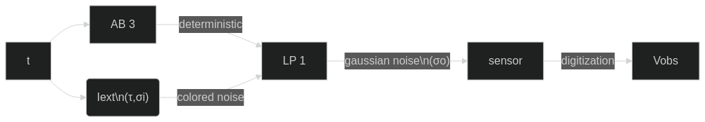
The model is composed of two neurons, AB and LP, with the AB neuron treated as part of the input: a known deterministic transformation of \(t\) into \(V_{\mathrm{AB}}\). However in the example traces we want to show the AB, so we create a equivalent model which actually returns the AB voltage trace. Since there is no connection back to AB, we only need to simulate the AB neuron.
raw_AB_model = Prinz2004(pop_sizes={"AB": 1}, g_ion=neuron_models.loc[[AB_model_label]],
                         gs=[[0]])
def AB_model(t_arr, I_ext=None, rng=None):
    res = raw_AB_model(t_arr, I_ext)
    series = res.V.loc[:,"AB"][1]
    series.name = "AB"
    return series
phys_models = Dict(
    true = CandidateModel("LP 1"),
    A    = CandidateModel("LP 2"),
    B    = CandidateModel("LP 3"),
    C    = CandidateModel("LP 4"),
    D    = CandidateModel("LP 5")
)
Generative observation model#
An observation model is a function which takes both the independent and dependent variables (generically \(x\) and \(y\)), and returns a transformed value \(\tilde{y}\). Processes which are time-independent (such as simple additive Gaussian noise) can simply ignore their \(x\) argument.
Using dataclasses is a simple way to allow binding parameters to a noise function. The pattern for defining a noise model is to use a dataclass, a pair of nested functions. The outer function sets the noise parameters, the inner function applies the noise to data:
(Using something like functools.partial to bind parameters would also work, but dataclasses self-document and serialize better.)
For consistency, noise arguments should always include a random number generator rng, even if the noise is actually deterministic. The value passed as rng should be a Generator instance, as created by numpy.random.default_rng or numpy.random.Generator.
@dataclass
class Digitizer:
    """Digitization noise model"""
    rng: RNGenerator|None=None
    def __call__(self, xy: "pd.Series", rng=None):
        rng = rng or self.rng
        return np.clip(xy, -128, 127).astype(np.int8)

@dataclass
class AdditiveNoise:
    """Additive noise model."""
    label: str
    σ    : PintQuantity
    μ    : PintQuantity    =0.*mV
    rng  : RNGenerator|None=None
    def __post_init__(self):  # Make sure μ & σ use the same units
        if self.μ != 0: self.μ = self.μ.to(self.units)
    @property
    def units(self):
        return getattr(self.σ, "units", mV)
    @property
    def rv(self):
        match self.label:
            case "Gaussian": return stats.norm(loc=self.μ.m, scale=self.σ.m)
            case "Cauchy": return stats.cauchy(loc=self.μ.m, scale=self.σ.m/2)
            case "Uniform": return stats.uniform(loc=self.μ.m-self.σ.m, scale=2*self.σ.m)
            case _: raise ValueError(f"Unrecognized noise label {self.label}")

    def __call__(self, xy: pd.Series, rng: np.random.Generator=None):
        rng = rng or self.rng
        return xy + self.rv.rvs(size=xy.shape, random_state=rng)
The three types of noise we consider – Gaussian, Cauchy and uniform – have been scaled so that for the same \(σ\) they have visually comparable width:
xarr = np.linspace(-3, 3, 200)
μ, σ = 0*mV, 1*mV
fig = hv.Overlay(
    [hv.Curve(zip(xarr, noise.rv.pdf(xarr)), label=noise.label).opts(color=color)
     for noise, color in zip([AdditiveNoise("Gaussian", σ, μ), AdditiveNoise("Cauchy", σ, μ), AdditiveNoise("Uniform", σ, μ)],
                             hv.Cycle("Dark2").values)]
)
# Plot styling
fig.opts(fig_inches=5, aspect=2, fontscale=1.3)

Full data model definition#
Our full data generating model is the LP1 physical model composed with Gaussian noise and digitization.
Important
The purpose attribute serves as our RNG seed.
We take care not to make the RNG itself an attribute: sending RN generators is fragile and memory-hungry, while sending seeds is cheap and easy.
Within the Calibrate task, each data model is shipped to an MP subprocess with pickle: by making Dataset callable, we can ship the Dataset instance (which only needs to serialize a seed) instead of the utils.compose instance (which would serialize an RNG)
@dataclass(frozen=True)
class Dataset:
    purpose: str
    L      : int
    τ      : PintQuantity  # Iext correlation time
    σi     : PintQuantity  # Iext strength
    obs_model: Literal["Gaussian","Uniform","Cauchy"]
    σo     : PintQuantity  # Observation noise strength
    LP_model: str="LP 1"

    def __post_init__(self):
        object.__setattr__(self, "_cached_data", None)
    @property
    def rng(self): return utils.get_rng("Prinz", self.purpose)
    @property
    def data_model(self):
        return utils.compose(
            Digitizer(),
            AdditiveNoise("Gaussian", μ=0*mV, σ=self.σo),
            DataModel(self.LP_model, noise_τ = self.τ, noise_σ = self.σi)
        )
    def get_data(self, rng=None):
        """Compute the data. MAY retrieve from in-memory cache, if `rng` is None."""
        # Implementing our own caching (instead of using lru_cache) avoids memory leaks: https://stackoverflow.com/questions/33672412/python-functools-lru-cache-with-instance-methods-release-object
        data = getattr(self, "_cached_data", None) if rng is None else None
        if data is None:
            data = self.__call__(self.L, rng)
            if rng is None:
                object.__setattr__(self, "_cached_data", data)
        return data
    def __call__(self, L, rng=None):
        return self.data_model(L, rng=(rng or self.rng))
Example traces#
Because holoviews can’t produce a grid layout with merged cells, we plot the circuit and the traces separately.
The full figure is full width, which is why we use a width of 2*config.fig_inches.
TODO: Aspect of the whole plot should be 50% flatter. For the current version, this was done in Inkscape. Sublabels should also be reduced.
Circuit panel
Show code cell source
import matplotlib.pyplot as plt
class DrawCircuit:
    def hvhook(self, xycolor, conn):
        """Creates a hook which can be used in a Holoviews plot"""
        def _hook(plot, element):
            self.__call__(xycolor, conn, plot.handles["axis"])
        return _hook
    def __call__(self, xycolor, conn, ax=None):
        r = 1  # node radius
        for x,y,ec,fc in xycolor:
            neuron = plt.Circle((x,y), r, edgecolor=ec, facecolor=fc)
            ax.add_patch(neuron)
        for i, j in conn:
            xyi = xycolor[i][:2]
            xyj = xycolor[j][:2]
            x, y = xycolor[i][:2]
            dx = xyj[0] - xyi[0]
            dy = xyj[1] - xyi[1]
            # Compute offsets so arrow starts/ends outside node circles
            θ = np.arctan2(dy, dx)
            ox = r*np.cos(θ)
            oy = r*np.sin(θ)
            ax.arrow(x+ox, y+oy, dx-2*(ox), dy-2*(oy),
                     length_includes_head=True, head_width=.4*r, head_length=.4*r,
                     edgecolor="black", facecolor="black")
draw_circuit = DrawCircuit()
circuit = hv.Scatter([(0,0)]).opts(color="none").opts(hooks=[viz.noaxis_hook])
circuit.opts(hooks=[draw_circuit.hvhook([(0,0, colors.AB, colors.AB_fill), (0,-3, colors.LP_data, colors.LP_data_fill)],
                                        [(0, 1)]),
                    viz.noaxis_hook
                   ]
            )

circuit_panel = circuit * hv.Text(0,0, "AB") * hv.Text(0,-3, "LP")
circuit_panel.opts(hv.opts.Text(weight="bold"))
xlim=(-1.5, 1.5); ylim=(-5, 1.5)
circuit_panel.opts(aspect=np.diff(xlim)/np.diff(ylim), xlim=xlim, ylim=ylim,
                   fig_inches=2*config.figures.defaults.fig_inches/4)  # 2*fig_inches for full width, /4 for four columns
circuit_panel

#viz.save(circuit_panel, config.paths.figures/"prinz_circuit_raw.pdf")
viz.save(circuit_panel, config.paths.figures/"prinz_circuit_raw.svg")
Trace panels
LP_data = Dataset(("example trace", "data"), L_data, LP_model="LP 1",
                  τ=data_Iext_τ, σi=data_Iext_σ, obs_model="Gaussian", σo=data_obs_σ)
LP_candidate_data = Dict(
    A = replace(LP_data, purpose=("example trace", "A"), LP_model="LP 2"),
    B = replace(LP_data, purpose=("example trace", "B"), LP_model="LP 3"),
    C = replace(LP_data, purpose=("example trace", "C"), LP_model="LP 4"),
    D = replace(LP_data, purpose=("example trace", "D"), LP_model="LP 5"),
)
AB_trace = AB_model(LP_data.get_data().index)
/home/alex/.cache/pypoetry/virtualenvs/emd-paper-8sT9_m0L-py3.11/lib64/python3.11/site-packages/scipy/integrate/_ivp/rk.py:109: RuntimeWarning: invalid value encountered in divide
  return norm(self._estimate_error(K, h) / scale)
Show code cell source
# Create scale bars
y0 = AB_trace.min()
Δy = AB_trace.max() - AB_trace.min()
x0 = AB_trace.index.min()
Δx = AB_trace.index.max() - AB_trace.index.min()
scaleargs = dict(kdims=["time"], vdims=["AB"], group="scale")
textargs  = dict(fontsize=8, kdims=["time", "AB"], group="scale")
scale_bar_time  = hv.Curve([(x0, y0-0.1*Δy), (x0+1000, y0-0.1*Δy)], **scaleargs)
scale_text_time = hv.Text(x0, y0-0.25*Δy, "1 s", halign="left", **textargs)
scale_bar_volt  = hv.Curve([(x0-0.065*Δx, y0), (x0-0.065*Δx, y0+50)], **scaleargs)
scale_text_volt = hv.Text(x0-0.14*Δx, y0, "50 mV", valign="bottom", rotation=90, **textargs)

# Assemble panels into layout
AB_data_panel = hv.Curve(AB_trace, group="Data", label="AB") * scale_bar_time * scale_text_time * scale_bar_volt * scale_text_volt
LP_data_panel = hv.Curve(LP_data.get_data(), group="Data", label="LP") * scale_bar_time * scale_bar_volt
LP_candidate_panels = [hv.Curve(LP_candidate_data[a].get_data(), group="Candidate", label="LP")
                       .opts(color=c)
                       * scale_bar_time * scale_bar_volt
                       for a, c in zip("ABCD", colors.LP_candidates.values)]
panels = [AB_data_panel, LP_data_panel, *LP_candidate_panels]

# Forcefully normalize the ranges (this *should* be done by Holoviews when axiswise=False, but it doesn’t seem to work
# – even for the time dimension, which is the same in each panel.
# This is important for the panels to be comparableqg
panels = [panel.redim.range(time=(2500, 7000), AB=(-85, 60), LP=(-85, 60))
          for panel in panels]

# Assemble panels into layout
layout = hv.Layout(panels)

# Plot styling
layout.opts(
    hv.opts.Overlay(show_legend=False, hooks=[viz.noaxis_hook]),
    hv.opts.Curve(hooks=[viz.noaxis_hook]), hv.opts.Curve(linewidth=1, backend="matplotlib"),
    hv.opts.Curve("Data.AB", color=colors.AB),
    hv.opts.Curve("Data.LP", color=colors.LP_data),
    #hv.opts.Curve("Candidate.LP", color=colors.LP_candidates),
    hv.opts.Curve("Scale", color=colors.scale), hv.opts.Curve("Scale", linewidth=1.5, backend="matplotlib"),
    hv.opts.Text("Scale", color=colors.scale),
    hv.opts.Layout(transpose=True, sublabel_position=(-.15, 0.6), sublabel_size=10, sublabel_format="({alpha})"),
    hv.opts.Layout(fig_inches=2*config.figures.defaults.fig_inches/4,
                   hspace=.2, vspace=0.1, backend="matplotlib")
).cols(2)

Loss functions#
Define loss functions for each candidate model. For simplicity here we fix the array of time stops to \([3000, 3001, \dotsc, 7000]\).
All candidate models assume Gaussian noise with \(σ = 2\), and we use the negative log likelihood for the loss:
where \(\hat{y}_a\) is the noise-free prediction from model \(a\).
Important
Observation models – like the Gaussian noise we assume here – are added by necessity: we mostly care about the physical model (here \(\Bspec_{\mathrm{RJ}}\) or \(\Bspec_{\mathrm{P}}\)), but since that doesn’t predict the data perfectly, we need the observation model to account for discrepancies. Therefore, barring a perfect physical model, a candidate model is generally composed of both:
(If the inputs to the physical model are also unknown, then the r.h.s. may also have a third input model term.)
The concrete takeaway is that to define the candidate models, we need to determine the value of \(σ\). Here we do this by maximizing the likelihood.
Important also is to tailor the observation model to the specifics of the system – consider for example the difference between testing a model using 1000 measurements from the same device, versus using 1000 single measurements from 1000 different devices. In the latter case, it might make more sense to use a posterior probability as an observation model.
On the appropriateness of maximum likelihood parameters
For simple models with a convex likelihood fitting parameters by maximizing the likelihood is often a good choice. We do this for illustrative reasons: since it it a common choice, it allows us to avoid sidetracking our argument with a discussion on the choice of loss. However, for time series, this choice tends to be over-sensitive to timing: consider a model which is almost correct, but with spikes slightly time shifted. Possibly more robust alternatives would a loss based on look-ahead probabilities (using the voltage trace of the data to predict the next observation) or averaging over many input realizations.
In general, more complex models tend to have a less regular likelihood landscape, with sharp peaks and deep valleys. Neural networks are one notorious example of a class of models with very sharp peaks in their likelihood. To illustrate one type of situation which can occur, consider the schematic log likelihood sketched below, where the parameter \(θ\) has highest likelihood when \(θ=3\). However, if there is uncertainty on that parameter, then the steep decline for \(θ>3\) would strongly penalize the risk. In contrast, the value \(θ=1\) is more robust against variations, and its risk less strongly penalized.

This sensitivity of the risk is exactly what the EMD criterion uses to assess candidate models. However it only does so for the selected candidate models – if we omit to include the best models in our candidate pool, the EMD won’t find them. Thus we should only use maximum likelihood parameters if we expect them to yield the best models.
Loss functions \(q\) typically only require the observed data as argument, so depending whether data_model returns \(x\) and \(y\) separately as x and y or as single object xy, the signature for \(q\) should be either
q(x, y)
or
q(xy)
Additional parameters can be fixed at definition time.
In this notebook our traces are stored as Pandas Series objects, so we use the q(xy) signature.
@dataclass
class Q:
    """Loss of a model assuming Gaussian observation noise.

    :param:phys_model: One of the keys in `phys_models`.
        Corresponding model is assumed deterministic.
    :param:obs_model: An instance of an observation model.
        Must have a `rv` attribute, providing access to the underlying distribution.
    """
    phys_model: Literal["LP 1", "LP 2", "LP 3", "LP 4", "LP 5"]
    obs_model: Literal["Gaussian", "Uniform", "Cauchy"]
    σ: float  # Allowed to be None at initialization, as long as it is set before __call__
    def __post_init__(self):
        if isinstance(self.phys_model, str):
            self._physmodel = CandidateModel(self.phys_model)
        else:
            assert isinstance(self.phys_model, CandidateModel)
            self._physmodel = self.phys_model
            self.phys_model = self.phys_model.LP_model
        self._obsmodel = AdditiveNoise(self.obs_model, self.σ)
    def __call__(self, xy: pd.Series):
        self._obsmodel.σ = self.σ
        ytilde = self._physmodel(xy)
        return -self._obsmodel.rv.logpdf(xy-ytilde)
Candidate models#
As mentioned above, the observation model parameters (here \(σ\)) are also part of the candidate models, so to construct candidate models we also need to set \(σ\). We do this by maximizing the likelihood of \(σ\).
The true observation model is not always the best
Generally speaking, even when the data are generated with discrete noise, candidate models should be assessed with a continuous noise model. Otherwise, any discrepancy between model and data would lead to an infinite risk. Likewise, an observation model with finite support (such as a uniform distribution) is often a poor choice, since data points outside that support will also cause the risk to diverge.
An exception this rule is when the image of the noise is known. For example, with the Digitizer noise, we know the recorded signal \(\bar{y}\) is rounded to the nearest integer from the actual voltage \(y\). We could include this in the candidate observation model, by inverting the model to get \(p(y \mid \bar{y})\). However we then would need to integrate this probability with the likelihood, which adds much computational cost, for a relatively small gain of precision in the fitted parameters.
On the flip side, some distributions are perfectly fine for fitting but make things more challenging when used to generate data. For example, when estimating the expected negative log likelihood from samples, the number of samples required is about 10x greater if they are generated from a Cauchy compared to a Normal distribution.
@lru_cache(maxsize=16)  # Don’t make this too large: each entry in the cache keeps a reference to `dataset` and `phys_model`, each of which maintains a largish cach, preventing it from being being deleted
def fit_gaussian_σ(dataset: Dataset, phys_model: str|CandidateModel, obs_model: str) -> float:
    """
    """
    data = dataset.get_data()
    _Q = Q(phys_model, obs_model=obs_model, σ=None)
    def f(log2_σ):
        _Q.σ = 2**log2_σ * mV
        risk = _Q(data).mean()
        # We could add priors here to regularize the fit, but there should be
        # enough noise in the data that this isn’t necessary.
        return risk

    res = optimize.minimize(f, np.log2(data_obs_σ.m), tol=1e-5)
    assert res.success
    return 2**res.x * mV
candidate_models = Dict()
Qrisk = Dict()
for a in "ABCD":
    fitted_σ = fit_gaussian_σ(LP_data, phys_models[a], "Gaussian")
    candidate_models[a] = utils.compose(AdditiveNoise("Gaussian", fitted_σ),
                                        phys_models[a])
    Qrisk[a] = Q(phys_model=phys_models[a], obs_model="Gaussian", σ=fitted_σ)
Candidate model PPFs#
Remark: Obtaining the PPF from samples is almost always easiest
Even though the error model here is just unbiased Gaussian noise, the PPF of the loss (i.e. the negative log likelihood) is still non-trivial to calculate. To see why, let’s start by considering how one might compute the CDF. Relabeling \(y\) to be the difference between observation and prediction, the (synthetic/theoretical) data are distributed as \(y \sim \mathcal{N}(0, σ)\). With the risk \(q = \log p(y)\), we get for the CDF of \(q\):
Substituting the probability of the Gaussian \(p(y) = \frac{1}{\sqrt{2πσ}} \exp(-y^2/2σ^2)\), we get
The result can be written in terms of error functions (by integrating the second term by parts to get rid of the \(y^2\)), but it’s not particularly elegant. And then we still need to invert the result to get \(q(Φ)\).
A physicist may be willing to make simplifying assumptions, but at that point we might as well use the approximate expression we get by estimating the PPF from samples.
All this to say that in the vast majority of cases, we expect that the most convenient and most accurate way to estimate the PPF will be to generate a set of samples and use make_empirical_risk_ppf.
In order to create a set of risk samples for each candidate model, we define for each a generative model which includes the expected noise (in this case additive Gaussian noise with parameter \(σ\) fitted above). For each model, we then generate a synthetic dataset, evaluate the risk \(q\) at every data point, and get a distribution for \(q\). We represent this distribution by its quantile function, a.k.a. point probability function (PPF).
def generate_synth_samples(model: CandidateModel, L_synth: int=L_synth,
                           Δt: float=data_Δt, t_burnin: float=data_burnin_time):
    rng = utils.get_rng("prinz", "synth_ppf", model[1].LP_model)
    tarr = data_burnin_time + np.arange(L_synth)*Δt
    return model(tarr, rng=rng)
Note
The synthetic PPFs for the \(A\) and \(B\) models are slightly but significantly below those of the \(C\) and \(D\) models. This is likely due to the slightly small \(σ\) obtained when fitting those models to the data.
synth_ppf = Dict({
    a: emd.make_empirical_risk_ppf(Qrisk[a](generate_synth_samples(candidate_models[a])))
    for a in "ABCD"
})
Show code cell source
Φarr = np.linspace(0, 1, 200)
curve_synth_ppfA = hv.Curve(zip(Φarr, synth_ppf.A(Φarr)), kdims=dims.Φ, vdims=dims.q, group="synth", label="synth PPF (model A)")
curve_synth_ppfB = hv.Curve(zip(Φarr, synth_ppf.B(Φarr)), kdims=dims.Φ, vdims=dims.q, group="synth", label="synth PPF (model B)")
curve_synth_ppfC = hv.Curve(zip(Φarr, synth_ppf.C(Φarr)), kdims=dims.Φ, vdims=dims.q, group="synth", label="synth PPF (model C)")
curve_synth_ppfD = hv.Curve(zip(Φarr, synth_ppf.D(Φarr)), kdims=dims.Φ, vdims=dims.q, group="synth", label="synth PPF (model D)")
fig_synth = curve_synth_ppfA * curve_synth_ppfB * curve_synth_ppfC * curve_synth_ppfD
# Plot styling
fig_synth.opts(hv.opts.Curve("synth", color=colors.LP_candidates),
               hv.opts.Overlay(show_title=False, legend_position="top_left"),
               hv.opts.Overlay(legend_position="right", fontscale=1.75),
               hv.opts.Overlay(fig_inches=4, backend="matplotlib"))

The EMD criterion works by comparing a synthetic PPF with a mixed PPF. The mixed PPF is obtained with the same risk function but evaluated on the actual data.
Compared to the synthetic PPFs, now see more marked differences between the PPFs of the different models.
If the theoretical models are good, differences between synthetic and mixed PPFs can be quite small. They may only be visible by zooming the plot. This is fine – in fact, models which are very close to each other are easier to calibrate, since it is easier to generate datasets for which either model is an equally good fit.
Note that the mixed PPF curves are above the synthetic ones. Although there are counter-examples (e.g. if a model overestimates the variance of the noise), this is generally expected, especially if models are fitted by minimizing the risk.
mixed_ppf = Dict(
    A = emd.make_empirical_risk_ppf(Qrisk.A(LP_data.get_data())),
    B = emd.make_empirical_risk_ppf(Qrisk.B(LP_data.get_data())),
    C = emd.make_empirical_risk_ppf(Qrisk.C(LP_data.get_data())),
    D = emd.make_empirical_risk_ppf(Qrisk.D(LP_data.get_data()))
)
Show code cell source
curve_mixed_ppfA = hv.Curve(zip(Φarr, mixed_ppf.A(Φarr)), kdims=dims.Φ, vdims=dims.q, group="mixed", label="mixed PPF (model A)")
curve_mixed_ppfB = hv.Curve(zip(Φarr, mixed_ppf.B(Φarr)), kdims=dims.Φ, vdims=dims.q, group="mixed", label="mixed PPF (model B)")
curve_mixed_ppfC = hv.Curve(zip(Φarr, mixed_ppf.C(Φarr)), kdims=dims.Φ, vdims=dims.q, group="mixed", label="mixed PPF (model C)")
curve_mixed_ppfD = hv.Curve(zip(Φarr, mixed_ppf.D(Φarr)), kdims=dims.Φ, vdims=dims.q, group="mixed", label="mixed PPF (model D)")
fig_emp = curve_mixed_ppfA * curve_mixed_ppfB * curve_mixed_ppfC * curve_mixed_ppfD
fig_emp.opts(hv.opts.Curve("mixed", color=colors.LP_candidates),
             hv.opts.Curve("mixed", linestyle="dashed", backend="matplotlib"),
             hv.opts.Curve("mixed", line_dash="dashed", backend="bokeh"))

fig = fig_synth * fig_emp
fig.opts(hv.opts.Overlay(legend_position="right", fontscale=1.75, fig_inches=4, backend="matplotlib"),
         hv.opts.Overlay(legend_position="right", width=600, backend="bokeh"))
hv.output(fig.redim.range(q=(-10, 200)), backend="bokeh")
Technical validity condition (WIP)
Caution
Something about this argument feels off; I need to think this through more carefully.
We can expect that the accuracy of a quantile function estimated from samples will be poorest at the extrema near \(Φ=0\) and \(Φ=1\): if we have \(L\) samples, than the “poorly estimated regions” are roughly \([0, \frac{1}{L+1})\) and \((\frac{L}{L+1}, 1]\). Our goal ultimate is to estimate the risk by computing the integral \(\int_0^1 q(Φ)\). The contribution of the low extremum region will scale like
and similarly for the high extremum region. Since we the estimated \(q\) function is unreliable within these regions, we their contribution to the full integral to become negligible once we have enough samples:
In other words, \(q\) may approx \(\pm \infty\) at the extrema, but must do so at a rate which is sublinear.
Interestingly, low-dimensional models like the 1-d examples studied in this work seem to be the most prone to superlinear growth of \(q\). This is because on low-dimensional distributions, the mode tends to be included in the typical set, while the converse is true in high-dimensional distributions (see e.g. chapter 4 of MacKay [46]). Nevertheless, we found that even in this case, the EMD distribution seems to assign plausible, and most importantly stable, distributions to the risk \(R\).
Where things get more dicey is with distributions with no finite moments. For example, if samples are generated by drawing from a Cauchy distribution, then the value of the function in the “poorly estimated region” remains, because as we draw more samples, we keep getting new samples with such enormous risk that they outweigh all the accumulated contributions up to that point. One solution in such cases may simply be to use a risk function which is robust with regards to outliers.
Hint
We recommend always inspecting quantile functions visually. For examples, if the risk function is continuous, then we expect the PPF to be smooth (since it involves integrating the risk) – if this isn’t the case, then we likely need more samples to get a reliable estimate
How many samples do we need ?#
Samples are used ultimately to estimate the risk. This is done in two ways:
By integrating the PPF.
By directly averaging the risk of each sample.
When computing the \(\Bemd{AB;c}\) criterion we use the first approach. During calibration we compare this with \(\Bconf{AB}\), which uses the second approach. When computing \(\Bconf{AB}\), we ideally use enough samples to reliably determine which of \(A\) or \(B\) has the highest risk.
In the figure below we show the risk as a function of the number of samples, computed either by constructing the PPF from samples and then integrating it (left) or averaging the samples directly (right). We see that models only start to differentiate at 4000 samples, and curves seem to flatten out around 20000.
The takeaway from this verification is that a value Linf=16384 should be sufficient for the calibration. Higher values might make \(\Bconf{}\) estimates still a bit more accurate, but at the cost of even longer integration times.
# # Reintegrating the model for every L would take a long time, so we integrate
# # once with the longest time, and then randomly select subsets of different sizes

LP_data_nsamples = replace(LP_data, L=40000, purpose=("prinz", "n samples ppf"))

# To save computation time, we reuse the samples used to compute the synthetic PPFs.
# Function results are cached to the disk, so if we use the same arguments, they are
# just read back instead of recomputed
q_samples = Dict(
    A = Qrisk.A(LP_data_nsamples.get_data()),
    B = Qrisk.B(LP_data_nsamples.get_data()),
    C = Qrisk.C(LP_data_nsamples.get_data()),
    D = Qrisk.D(LP_data_nsamples.get_data())
    # A = Qrisk.A(generate_synth_samples(candidate_models["A"])),
    # B = Qrisk.B(generate_synth_samples(candidate_models["B"])),
    # C = Qrisk.C(generate_synth_samples(candidate_models["C"])),
    # D = Qrisk.D(generate_synth_samples(candidate_models["D"]))
)
Rvals_ppf = {"A": {}, "B": {}, "C": {}, "D": {}}
Rvals_avg = {"A": {}, "B": {}, "C": {}, "D": {}}
nsamples_rng = utils.get_rng("prinz", "nsamples")
for model in Rvals_ppf:
    for _L in np.logspace(2, 4.6, 30):  # log10(40000) = 4.602
        _L = int(_L)
        if _L % 2 == 0: _L+=1  # Ensure L is odd
        q_list = nsamples_rng.choice(q_samples[model], _L)  # Bootstrap sampling with replacement
        ppf = emd.make_empirical_risk_ppf(q_list)
        Φ_arr = np.linspace(0, 1, _L+1)
        Rvals_ppf[model][_L] = integrate.simpson(ppf(Φ_arr), x=Φ_arr)
        Rvals_avg[model][_L] = q_list.mean()
Show code cell source
curves = {"ppf": [], "avg": []}
for model in "ABCD":
    curves["ppf"].append(
        hv.Curve(list(Rvals_ppf[model].items()),
                 kdims=hv.Dimension("L", label="num. samples"),
                 vdims=hv.Dimension("R", label="exp. risk"),
                 label=f"model {model} - true samples"))
    curves["avg"].append(
        hv.Curve(list(Rvals_avg[model].items()),
                 kdims=hv.Dimension("L", label="num. samples"),
                 vdims=hv.Dimension("R", label="exp. risk"),
                 label=f"model {model} - true samples"))
fig_ppf = hv.Overlay(curves["ppf"]).opts(title="Integrating $q$ PPF")
fig_avg = hv.Overlay(curves["avg"]).opts(title="Averaging $q$ samples")
fig_ppf.opts(show_legend=False)
fig = fig_ppf + fig_avg
# Plot styling
fig.opts(
    hv.opts.Overlay(logx=True, fig_inches=5, aspect=3, fontscale=1.7, legend_position="right", backend="matplotlib")
)

Calibration#
Epistemic distributions#
Calibration is a way to test that \(\Bemd{AB;c}\) actually does provide a bound on the probability that \(R_A < R_B\), where the probability is over a variety of experimental conditions.
There is no unique distribution over experimental conditions, so what we do is define many such distributions; we refer to these as epistemic distributions. Since calibration results depend on the model, we repeat the calibration for different pairs \((a,b)\) of candidate models – of the six possible pairs, we select three: \((A,B)\), \((A,C)\) and \((C,D)\).
We look for a value of \(c\) which is satisfactor with all epistemic distributions. Here knowledge of the system being modelled is key: for any given \(c\), it is always possible to define an epistemic distribution for which calibration fails – for example, a model which is 99% random noise would be difficult to calibrate against. The question is whether the uncertainty on experimental conditions justifies including such a model in our distribution. Epistemic distributions are how we quantify our uncertainty in experimental conditions, or describe what we think are reasonable variations of those conditions.
The epistemic distributions are defined in Section 4.4.2 and repeated here for convenience. (In the expressions below, \(ξ\) denotes the noise added to the voltage \(V^{\mathrm{LP}}\).)
Important
Calibration is concerned with the transition from “certainty in model \(A\)” to “equivocal evidence” to “certainty in model \(B\)”. It is of no use to us if all calibration datasets are best fitted with the same model. The easiest way to avoid this is to use the candidate models to generate the calibration datasets, randomly selecting which candidate is used for each dataset. All other things being equal, the calibration curve will resolve fastest if we select each candidate with 50% probability.
We also need datasets to span the entire range of certainties, with both clear and ambiguous decisions in favour of \(A\) or \(B\). One way to do this is to start from a dataset where the models are easy to discriminate, and identify a control parameter which progressively makes the discrimination more ambiguous. In this example, we started with a dataset with no external input \(I_{ext}\) – the model is then perfectly deterministic, and \(\Bemd{}\) almost always either 0 or 1. We can then adjust the strength of \(I_{ext}\) to transition from perfect certainty to perfect confusion. Alternatively, we could start from a dataset with near-perfect confusion, and identify a control parameters which makes the decision problem less ambiguous – this is what we do in the ultraviolet castastrophe example.
Note that since we use the candidate models to generate the datasets during calibration, we don’t need to know the true data model. We only need to identify a regime where model predictions differ.
We can conclude from these remarks that calibration works best when the models are close and allow for ambiguity. However this is not too strong a limitation: if we are unable to calibrate the \(\Bemd{}\) because there is no ambiguity between models, then we probability don’t need the \(\Bemd{}\) to determine which one to reject.
Observation noise model
One of Gaussian or Cauchy. The distributions are centered and \(σ_o\) is drawn from the distribution defined below. Note that this is the model used to generate data. The candidate models always evaluate their loss assuming a Gaussian observation model.
Gaussian: \(\begin{aligned}p(ξ) &= \frac{1}{\sqrt{2πσ}} \exp\left(-\frac{ξ^2}{2σ_o^2}\right) \end{aligned}\)
Cauchy: \(\begin{aligned} p(ξ) = \frac{2}{πσ \left[ 1 + \left( \frac{ξ^2}{σ_o/2} \right) \right]} \end{aligned}\)
Observation noise strength \(σ_o\)
Low noise: \(\log σ_o \sim \nN(0.0 \mathrm{mV}, (0.5 \mathrm{mV})^2)\)
High noise: \(\log σ_o \sim \nN(1.0 \mathrm{mV}, (0.5 \mathrm{mV})^2)\)
External input strength \(σ_i\)
The parameter \(σ_i\) sets the strength of the input noise such that \(\langle{I_{\mathrm{ext}}^2\rangle} = σ_i^2\).
Weak input: \(\log σ_i \sim \nN(-15.0 \mathrm{mV}, (0.5 \mathrm{mV})^2)\)
Strong input: \(\log σ_i \sim \nN(-10.0 \mathrm{mV}, (0.5 \mathrm{mV})^2)\)
External input correlation time \(τ\)
The parameter \(σ_i\) sets the correlation time of the input noise such that \(\langle{I_{\mathrm{ext}}(t)I_{\mathrm{ext}}(t+s)\rangle} = σ_i^2 e^{s^2/2τ^2}\).
Short correlations: \(\log_{10} τ \sim \Unif([0.1 \mathrm{ms}, 0.2 \mathrm{ms}])\)
Long correlation: \(\log_{10} τ \sim \Unif([1.0 \mathrm{ms}, 2.0 \mathrm{ms}])\)
We like to avoid Gaussian distributions for calibration, because often Gaussian are “too nice”, and may hide or suppress rare behaviours. (For example, neural network weights are often not initialized with Gaussians: distributions with heavier tails tend to produce more exploitable initial features.) Uniform distributions are convenient because they can produce extreme values with high probability, without also producing unphysically extreme values. This is of course only a choice, and in many cases a Gaussian calibration distribution can also be justified.
@dataclass(frozen=True)  # NB: Does not prevent use of @cached_property
class Experiment:        #     See https://docs.python.org/3/faq/programming.html#how-do-i-cache-method-calls
    a      : str
    b      : str
    dataset: Dataset

    @property
    def a_phys(self): return "LP "+{"A":"2", "B":"3", "C":"4", "D":"5"}[self.a]
    @property
    def b_phys(self): return "LP "+{"A":"2", "B":"3", "C":"4", "D":"5"}[self.b]

    # NB: We don’t use @property@cache because that creates a class-wide cache,
    #     which will horde memory. Instead, with @cached_property, the cache is
    #     tied to the instance, which can be freed once the instance is deleted.

    @cached_property
    def σa(self):
        return fit_gaussian_σ(self.dataset, self.a_phys, "Gaussian")
    @cached_property
    def σb(self):
        return fit_gaussian_σ(self.dataset, self.b_phys, "Gaussian")

    @property
    def data_model(self):
        return self.dataset
    @cached_property
    def candidateA(self):
        rnga = rng=utils.get_rng(*self.dataset.purpose, "candidate a")
        return utils.compose(AdditiveNoise("Gaussian", self.σa),
                             phys_models[self.a])
    @cached_property
    def candidateB(self):
        rngb = rng=utils.get_rng(*self.dataset.purpose, "candidate b")
        return utils.compose(AdditiveNoise("Gaussian", self.σb),
                             phys_models[self.b])
    @cached_property
    def QA(self):
        return Q(phys_models[self.a], "Gaussian", σ=self.σa)
    @cached_property
    def QB(self):
        return Q(phys_models[self.b], "Gaussian", σ=self.σb)
@dataclass(frozen=True)  # frozen allows dataclass to be hashed
class EpistemicDist(emd.tasks.EpistemicDist):
    N: int|Literal[np.inf]

    a: Literal["A", "B", "C", "D"]
    b: Literal["A", "B", "C", "D"]
    ξ_name: Literal["Gaussian", "Cauchy", "Uniform"]  # Dataset observation model (not of candidates)
    σo_dist: Literal["low noise", "high noise"]
    τ_dist: Literal["no Iext", "short input correlations", "long input correlations"]
    σi_dist: Literal["no Iext", "weak input", "strong input"]

    # Hyperparameters
    τ_short_min   : PintQuantity=  0.1*ms
    τ_short_max   : PintQuantity=  0.2*ms
    τ_long_min    : PintQuantity=  1. *ms
    τ_long_max    : PintQuantity=  2. *ms
    σo_low_mean   : PintQuantity=  0. *mV
    σo_high_mean  : PintQuantity=  1. *mV
    σo_std        : PintQuantity=  0.5*mV
    σi_weak_mean  : PintQuantity=-15. *mV
    σi_strong_mean: PintQuantity=-10. *mV
    σi_std        : PintQuantity=  0.5*mV

    @property
    def a_phys(self): return "LP "+{"A":"2", "B":"3", "C":"4", "D":"5"}[self.a]
    @property
    def b_phys(self): return "LP "+{"A":"2", "B":"3", "C":"4", "D":"5"}[self.b]

    ## Standardization of arguments ##

    def __post_init__(self):
        # Standardize `a` and `b` models so `a < b`
        assert self.a != self.b, "`a` and `b` candidate models are the same"
        if self.a > self.b:
            a, b = self.a, self.b
            object.__setattr__(self, "a", b)
            object.__setattr__(self, "b", a)
        # Make sure all hyper parameters use expected units
        for hyperω in ["σo_low_mean" , "σo_high_mean"  , "σo_std",
                       "σi_weak_mean", "σi_strong_mean", "σi_std"]:
            object.__setattr__(self, hyperω, getattr(self, hyperω).to(mV))
        for hyperω in ["τ_short_min", "τ_short_max", "τ_long_min", "τ_long_max"]:
            object.__setattr__(self, hyperω, getattr(self, hyperω).to(ms))

    ## Replace  distribution labels with computable objects ##

    def get_physmodel(self, rng):
        return rng.choice([self.a_phys, self.b_phys])

    def get_τ(self, rng):
        match self.τ_dist:
            case "no Iext":
                return None
            case "short input correlations":
                return 10**rng.uniform(self.τ_short_min.m, self.τ_short_max.m) * ms
            case "long input correlations":
                return 10**rng.uniform(self.τ_long_min.m, self.τ_long_max.m) * ms
            case _:
                raise ValueError(f"Unrecognized descriptor '{_}' for `τ_dist`.")

    def get_σo(self, rng):
        match self.σo_dist:
            case "low noise":
                return rng.lognormal(self.σo_low_mean.m, self.σo_std.m) * mV
            case "high noise":
                return rng.lognormal(self.σo_high_mean.m, self.σo_std.m) * mV
            case _:
                raise ValueError(f"Unrecognized descriptor '{_}' for `σo_dist`.")

    def get_σi(self, rng):
        match self.σi_dist:
            case "no Iext":
                return 0
            case "weak input":
                #return rng.lognormal(-7, 0.5) * mV
                return rng.lognormal(self.σi_weak_mean.m, self.σi_std.m) * mV
            case "strong input":
                #return rng.lognormal(-5, 0.5) * mV
                return rng.lognormal(self.σi_strong_mean.m, self.σi_std.m) * mV
            case _:
                raise ValueError(f"Unrecognized descriptor '{_}' for `σi_dist`.")

    ## Experiment generator ##

    def __iter__(self):
        rng = utils.get_rng("prinz", "calibration",  self.a, self.b,
                            self.ξ_name, self.σo_dist, self.τ_dist, self.σi_dist)
        for n in range(self.N):
            dataset = Dataset(
                ("prinz", "calibration", "fit candidates", n),
                L = L_data,
                # Calibration parameters
                obs_model = self.ξ_name,
                # Calibration RVs
                LP_model = self.get_physmodel(rng),
                τ = self.get_τ(rng),
                σi = self.get_σi(rng),
                σo = self.get_σo(rng)
            )
            yield Experiment(self.a, self.b, dataset)

    def __getitem__(self, key):
        from numbers import Integral
        if not (isinstance(key, Integral) and 0 <= key < self.N):
            raise ValueError(f"`key` must be an integer between 0 and {self.N}. Received {key}")
        for n, D in enumerate(self):
            if n == key:
                return D
Execution#
How many experiments
The function emd.viz.calibration_plot attempts to collect results into 16 bins, so making \(N\) a multiple of 16 works nicely. (With the constraint that no bin can have less than 16 points.)
For an initial pilot run, we found \(N=64\) or \(N=128\) to be good numbers. These numbers produce respectively 4 or 8 bins, which is often enough to check that \(\Bemd{}\) and \(\Bconf{}\) are reasonably distributed and that the epistemic distribution is actually probing the transition from strong to equivocal evidence. A subsequent run with \(N \in \{256, 512, 1024\}\) can then refine and smooth the curve.
N = 512
Ωdct = {(f"{Ω.a} vs {Ω.b}", Ω.ξ_name, Ω.σo_dist, Ω.τ_dist, Ω.σi_dist): Ω
        for Ω in (EpistemicDist(N, a, b, ξ_name, σo_dist, τ_dist, σi_dist)
                  for (a, b) in [("A", "B"), ("A", "D"), ("C", "D")]
                  for ξ_name in ["Gaussian", "Cauchy"]
                  for σo_dist in ["low noise", "high noise"]
                  for τ_dist in ["short input correlations", "long input correlations"]
                  for σi_dist in ["weak input", "strong input"]
            )
       }
Note
The code cell above runs a large number of tasks, which took many days on a small server. For our initial run we selected specifically the 6 runs we wanted to appear in the the main text:
#N = 64
N = 512
Ωdct = {(f"{Ω.a} vs {Ω.b}", Ω.ξ_name, Ω.σo_dist, Ω.τ_dist, Ω.σi_dist): Ω
        for Ω in [
            EpistemicDist(N, "A", "D", "Gaussian", "low noise", "short input correlations", "weak input"),
            EpistemicDist(N, "C", "D", "Gaussian", "low noise", "short input correlations", "weak input"),
            EpistemicDist(N, "A", "B", "Gaussian", "low noise", "short input correlations", "weak input"),
            EpistemicDist(N, "A", "D", "Gaussian", "low noise", "short input correlations", "strong input"),
            EpistemicDist(N, "C", "D", "Gaussian", "low noise", "short input correlations", "strong input"),
            EpistemicDist(N, "A", "B", "Gaussian", "low noise", "short input correlations", "strong input"),
        ]
       }
Hint
Calibrate will iterate over its experiments argument twice, so it is important that Ωdct not be consumable.
tasks = {}
for Ωkey, Ω in Ωdct.items():
    task = emd.tasks.Calibrate(
        reason = f"Prinz calibration – {Ω.a} vs {Ω.b} - {Ω.ξ_name} - {Ω.σo_dist} - {Ω.τ_dist} - {Ω.σi_dist} - {N=}",
        #c_list = [.5, 1, 2],
        #c_list = [2**-8, 2**-7, 2**-6, 2**-5, 2**-4, 2**-3, 2**-2, 2**-1, 2**0],
        #c_list = [2**-8, 2**-6, 2**-4, 2**-2, 1],  # 60h runs
        #c_list = [2**0],
        #c_list = [2**-4, 2**0, 2**4],
        c_list = [2**-6, 2**-4, 2**-2, 2**0, 2**4],
        # Collection of experiments (generative data model + candidate models)
        experiments = Ω.generate(N),
        # Calibration parameters
        Ldata = L_data,
        #Linf = 12288  # 2¹³ + 2¹²
        #Linf = 32767 # 2¹⁵ - 1
        #Linf = 4096
        Linf = Linf
    )
    tasks[Ωkey]=task
The code below creates task files which can be executed from the command line with the following:
smttask run -n1 --import config <task file>
    for key, task in tasks.items():
        if not task.has_run:  # Don’t create task files for tasks which have already run
            Ω = task.experiments
            taskfilename = f"prinz_calibration__{Ω.a}vs{Ω.b}_{Ω.ξ_name}_{Ω.σo_dist}_{Ω.τ_dist}_{Ω.σi_dist}_N={Ω.N}_c={task.c_list}"
            task.save(taskfilename)
Analysis#
We can check the efficiency of sampling by plotting histograms of \(\Bemd{}\) and \(\Bconf{}\): ideally the distribution of \(\Bemd{}\) is flat, and that of \(\Bconf{}\) is equally distributed between 0 and 1. Since we need enough samples at every subinterval of \(\Bemd{}\), it is the most sparsely sampled regions which determine how many calibration datasets we need to generate. (And therefore how long the computation needs to run.) Beyond making for shorter compute times, a flat distribution however isn’t in and of itself a good thing: more important is that the criterion is able to resolve the models when it should.
c_chosen = 2**-2
c_list = [2**-6, 2**-4, 2**-2, 2**0, 2**4]
class CalibHists:
    def __init__(self, hists_emd=None, hists_conf=None):
        frames = {viz.format_pow2(c): hists_emd[c] * hists_conf[c] for c in hists_emd}
        self.hmap = hv.HoloMap(frames, kdims=["c"])
        self.hists_emd  = hists_emd
        self.hists_conf = hists_conf

def calib_hist(task) -> CalibHists:
    calib_results = task.unpack_results(task.run())

    hists_emd = {}
    hists_conf = {}
    for c, res in calib_results.items():
        hists_emd[c] = hv.Histogram(np.histogram(res["Bemd"], bins="auto", density=False), kdims=["Bemd"], label="Bemd")
        hists_conf[c] = hv.Histogram(np.histogram(res["Bconf"].astype(int), bins="auto", density=False), kdims=["Bconf"], label="Bconf")
    #frames = {viz.format_pow2(c): hists_emd[c] * hists_conf[c] for c in hists_emd}

    #hmap = hv.HoloMap(frames, kdims=["c"])
    hists = CalibHists(hists_emd=hists_emd, hists_conf=hists_conf)
    hists.hmap.opts(
        hv.opts.Histogram(backend="bokeh",
                          line_color=None, alpha=0.75,
                          color=hv.Cycle(values=config.figures.colors.light.cycle)),
        hv.opts.Histogram(backend="matplotlib",
                          color="none", edgecolor="none", alpha=0.75,
                          facecolor=hv.Cycle(values=config.figures.colors.light.cycle)),
        hv.opts.Overlay(backend="bokeh", legend_position="top", width=400),
        hv.opts.Overlay(backend="matplotlib", legend_position="top", fig_inches=4)
    )
    #hv.output(hmap, backend="bokeh", widget_location="right")
    return hists
def panel_calib_hist(task, c_list: list[float]) -> hv.Overlay:
    hists_hmap = calib_hist(task)

    _hists_emd = {c: h.relabel(group="Bemd", label=f"$c={viz.format_pow2(c, format='latex')}$")
                  for c, h in hists_hmap.hists_emd.items() if c in c_list}
    for c in c_list:
        α = 1 if c == c_chosen else 0.8
        _hists_emd[c].opts(alpha=α)
    histpanel_emd = hv.Overlay(_hists_emd.values())

    histpanel_emd.redim(Bemd=dims.Bemd, Bconf=dims.Bconf, c=dims.c)

    histpanel_emd.opts(
        hv.opts.Histogram(backend="matplotlib", color="none", edgecolor="none", facecolor=colors.calib_curves),
        hv.opts.Histogram(backend="bokeh", line_color=None, fill_color=colors.calib_curves),
        hv.opts.Overlay(backend="matplotlib",
                        legend_cols=3,
                        legend_opts={"columnspacing": .5, "alignment": "center",
                                     "loc": "upper center"},
                        hooks=[viz.yaxis_off_hook, partial(viz.despine_hook(), left=True)]),
        hv.opts.Overlay(backend="bokeh",
                        legend_cols=3),
        hv.opts.Overlay(backend="matplotlib",
                        fig_inches=config.figures.defaults.fig_inches,
                        aspect=1, fontscale=1.3,
                        xlabel="$B^{\mathrm{EMD}}$", ylabel="$B^{\mathrm{conf}}$",
                        ),
        hv.opts.Overlay(backend="bokeh",
                        width=4, height=4)
    )

    return histpanel_emd
Hint
Default options of calibration_plot can be changed by updating the configuration object config.emd.viz.matplotlib (relevant fields are calibration_curves, prohibited_areas, discouraged_area).
As with any HoloViews plot element, they can also be changed on a per-object basis by calling their .opts method.
def panel_calib_curve(task, c_list: list[float]) -> hv.Overlay:
    calib_results = task.unpack_results(task.run())
    calib_plot = emd.viz.calibration_plot(calib_results)

    calib_curves, prohibited_areas, discouraged_areas = calib_plot

    for c, curve in calib_curves.items():
        calib_curves[c] = curve.relabel(label=f"$c={viz.format_pow2(c, format='latex')}$")

    for c in c_list:
        α = 1 #if c == c_chosen else 0.85
        #w = 3 if c == c_chosen else 2
        w = 2
        calib_curves[c].opts(alpha=α, linewidth=w)

    curve_panel = prohibited_areas * discouraged_areas * hv.Overlay(calib_curves.select(c=c_list).values())

    curve_panel.redim(Bemd=dims.Bemd, Bconf=dims.Bconf, c=dims.c)

    # NB: When previously set options don’t specify `backend`, setting a 'bokeh' option can unset a previously set 'matplotlib' one
    curve_panel.opts(
        hv.opts.Curve(backend="matplotlib", color=colors.calib_curves),
        hv.opts.Curve(backend="bokeh", color=colors.calib_curves, line_width=3),
        hv.opts.Area(backend="matplotlib", alpha=0.5),
        #hv.opts.Area(backend="bokeh", alpha=0.5),
        hv.opts.Overlay(backend="matplotlib", legend_position="top_left", legend_cols=1, hooks=[viz.despine_hook]),
        hv.opts.Overlay(backend="bokeh", legend_position="top_left", legend_cols=1),
        hv.opts.Overlay(backend="matplotlib",
                        fig_inches=config.figures.defaults.fig_inches,
                        aspect=1, fontscale=1.3,
                        xlabel="$B^{\mathrm{EMD}}$", ylabel="$B^{\mathrm{conf}}$",
                        ),
        hv.opts.Overlay(backend="bokeh",
                        width=4, height=4)
    )

    return curve_panel
task = tasks['C vs D', 'Gaussian', 'low noise', 'short input correlations', 'weak input']
assert task.has_run
hv.output(calib_hist(task).hmap,
          backend="bokeh", widget_location="right")
Hint: Diagnosing \(\Bemd{}\) and \(\Bconf{}\) histograms
- \(\Bemd{}\) distribution which bulges around 0.5.
May indicate that \(c\) is too large and the criterion underconfident.
May also indicate that the calibration distribution is generating a large number of (
data,modelA,modelB) triples which are essentially undecidable. If neither model is a good fit to the data, then their \(δ^{\mathrm{EMD}}\) discrepancies between mixed and synthetic PPFs will be large, and they will have broad distributions for the risk. Broad distributions overlap more, hence the skew of \(\Bemd{}\) towards 0.5.- \(\Bemd{}\) distribution which is heavy at both ends.
May indicate that \(c\) is too small and the criterion overconfident.
May also indicate that the calibration distribution is not sampling enough ambiguous conditions. In this case the answer is not to increase the value of \(c\) but rather to tighten the calibration distribution to focus on the area with \(\Bemd{}\) close to 0.5. It may be possible to simply run the calibration longer until there have enough samples everywhere, but this is generally less effective than adjusting the calibration distribution.
- \(\Bemd{}\) distribution which is heavily skewed either towards 0 or 1.
Check that the calibration distribution is using both candidate models to generate datasets. The best is usually to use each candidate to generate half of the datasets: then each model should fit best in roughly half the cases. The skew need not be removed entirely – one model may just be more permissive than the other.
This can also happen when \(c\) is too small.
- \(\Bconf{}\) distribution which is almost entirely on either 0 or 1.
Again, check that the calibration distribution is using both models to generate datasets.
If each candidate is used for half the datasets, and we still see ueven distribution of \(\Bconf{}\), then this can indicate a problem: it means that the ideal measure we are striving towards (true risk) is unable to identify that model used to generate the data. In this case, tweaking the \(c\) value is a waste of time: the issue then is with the problem statement rather than the \(\Bemd{}\) calibration. Most likely the issue is that the loss is ill-suited to the problem:
It might not account for rotation/translation symmetries in images, or time dilation in time-series.
One model’s loss might be lower, even on data generated with the other model. This can happen with a log posterior, when one model has more parameters: its higher dimensional prior “dilutes” the likelihood. This may be grounds to reject the more complex model on the basis of preferring simplicity, but it is not grounds to falsify that model. (Since it may still fit the data equally well.)
#task = calib_tasks_to_show[0]
histpanel_emd = panel_calib_hist(task, c_list).opts(show_legend=False)
curve_panel = panel_calib_curve(task, c_list)
fig = curve_panel << hv.Empty() << histpanel_emd

calib_results = task.unpack_results(task.run())
calib_plot = emd.viz.calibration_plot(calib_results)  # Used below

fig.opts(backend="matplotlib", fig_inches=5)

Hint: Diagnosing calibration curves
- Flat calibration curve
This is the most critical issue, since it indicates that \(\Bemd{}\) is actually not predictive of \(\Bconf{}\) at all. The most common reason is a mistake in the definition of the calibration distribution, where some values are fixed when they shouldn’t be.
Remember that the model construction pipeline used on the real data needs to be repeated in full for each experimental condition produced by the calibration distribution. For example, in
Experimentabove we refit the observation noise \(σ\) for each experimental condition generated within__iter__.Treat any global used within
EpistemicDistwith particular suspicion, as they are likely to fix values which should be variable. To minimize the risk of accidental global variables, you can defineEpistemicDistin its own separate module.
To help investigate issues, it is often helpful to reconstruct conditions that produce the unexpected behaviour. The following code snippet recovers the first calibration dataset for which both
Bemd > 0.9andBconf = False; the recovered dataset isD:Bemd = calib_results[1.0]["Bemd"] Bconf = calib_results[1.0]["Bconf"] i = next(iter(i for i in range(len(Bemd)) if Bemd[i] > 0.9)) for j, D in zip(range(i+1), task.models_Qs): pass assert j == i
- Calibration curve with shortened domain
I.e. \(\Bemd{}\) values don’t reach 0 and/or 1. This is not necessarily critical: the calibration distribution we want to test may simply not allow to fully distinguish the candidate models under any condition.
If it is acceptable to change the calibration distribution (or to add one to the test suite), then the most common way to address this is to ensure the distribution produces conditions where \(\Bemd{}\) can achieve maximum confidence – for example by having conditions with negligeable observation noise.
Calibration figure: main text#
Show code cell source
tasks_to_show = [tasks[key] for key in [
    ('A vs B', 'Gaussian', 'low noise', 'short input correlations', 'weak input'),
    ('A vs B', 'Gaussian', 'low noise', 'short input correlations', 'strong input'),
    ('C vs D', 'Gaussian', 'low noise', 'short input correlations', 'weak input'),
    ('C vs D', 'Gaussian', 'low noise', 'short input correlations', 'strong input'),
    ('A vs D', 'Gaussian', 'low noise', 'short input correlations', 'weak input'),
    ('A vs D', 'Gaussian', 'low noise', 'short input correlations', 'strong input'),
]]
assert all(task.has_run for task in tasks_to_show), "Run the calibration tasks from the command line environment, using `smttask run`. Executing it as part of a Jupyter Book build would take a **long** time."
panels = [panel_calib_curve(task, c_list) for task in tasks_to_show]
panels[0].opts(title="$\\mathcal{{M}}_C$ vs $\\mathcal{{M}}_D$")
panels[2].opts(title="$\\mathcal{{M}}_A$ vs $\\mathcal{{M}}_B$")
panels[4].opts(title="$\\mathcal{{M}}_A$ vs $\\mathcal{{M}}_D$")
panels[0].opts(ylabel=r"weak $I_{\mathrm{ext}}$")
panels[1].opts(ylabel=r"strong $I_{\mathrm{ext}}$")
panels[0].opts(hv.opts.Overlay(legend_cols=5, legend_position="top_left", # Two placement options
                                legend_opts={"columnspacing": 2.}))
panels[4].opts(hv.opts.Overlay(legend_cols=1, legend_position="right"))    # for the shared legend
for i in (1, 2, 3, 4, 5):
    panels[i].opts(hv.opts.Overlay(show_legend=False))
for i in (0, 1, 2, 4, 5):
    panels[i].opts(xlabel="")
hooks = {i: [viz.despine_hook, viz.set_xticks_hook([0, 0.5, 1]), viz.set_yticks_hook([0, 0.5, 1])] for i in range(6)}
for i in (0, 1):
    hooks[i].extend([viz.set_yticklabels_hook(["$0$", "$0.5$", "$1$"])])
for i in (1, 3, 5):
    hooks[i].extend([viz.set_xticklabels_hook(["$0$", "$0.5$", "$1$"])])
for i, hook_lst in hooks.items():
    panels[i].opts(hooks=hook_lst)
    # panels[i].opts(hooks=[viz.set_yticks_hook([0, 0.5, 1]), viz.set_yticklabels_hook(["$0$", "$0.5$", "$1$"]), viz.despine_hook])
for i in (0, 2, 4):
    panels[i].opts(xaxis="bare")
for i in (2, 3, 4, 5):
    panels[i].opts(yaxis="bare")
# for i in (1, 3, 5):
#     panels[i].opts(hooks=[viz.set_xticks_hook([0, 0.5, 1]), viz.set_xticklabels_hook(["$0$", "$0.5$", "$1$"]), viz.despine_hook])
fig_calibs = hv.Layout(panels)
fig_calibs.opts(
    hv.opts.Layout(backend="matplotlib", sublabel_format="", #sublabel_format="({alpha})",
                   transpose=True,
                   fig_inches=0.4*config.figures.defaults.fig_inches,  # Each panel is 1/3 of column width. Natural width of plot is a bit more; we let LaTeX scale the image down a bit (otherwise we would need to tweak multiple values like font scales & panel spacings)
                   hspace=-0.25, vspace=0.2, tight=False
                  )
).cols(2)
hv.output(fig_calibs)

# Print panel descriptions
from tabulate import tabulate
headers = ["models", "input corr", "input strength", "obs noise", "obs dist"]
data = [(f"Panel ({lbl})",
         f"{(Ω:=task.experiments).a} vs {Ω.b}", f"{Ω.τ_dist}", f"{Ω.σi_dist}", f"{Ω.σo_dist}", f"{Ω.ξ_name} noise")
        for lbl, task in zip("abcdef", tasks_to_show)]
print(tabulate(data, headers, tablefmt="simple_outline"))

┌───────────┬──────────┬──────────────────────────┬──────────────────┬─────────────┬────────────────┐
│           │ models   │ input corr               │ input strength   │ obs noise   │ obs dist       │
├───────────┼──────────┼──────────────────────────┼──────────────────┼─────────────┼────────────────┤
│ Panel (a) │ A vs B   │ short input correlations │ weak input       │ low noise   │ Gaussian noise │
│ Panel (b) │ A vs B   │ short input correlations │ strong input     │ low noise   │ Gaussian noise │
│ Panel (c) │ C vs D   │ short input correlations │ weak input       │ low noise   │ Gaussian noise │
│ Panel (d) │ C vs D   │ short input correlations │ strong input     │ low noise   │ Gaussian noise │
│ Panel (e) │ A vs D   │ short input correlations │ weak input       │ low noise   │ Gaussian noise │
│ Panel (f) │ A vs D   │ short input correlations │ strong input     │ low noise   │ Gaussian noise │
└───────────┴──────────┴──────────────────────────┴──────────────────┴─────────────┴────────────────┘
viz.save(fig_calibs, config.paths.figures/"prinz_calibrations_raw.svg")
#viz.save(fig_calib.opts(fig_inches=5.5/3, backend="matplotlib", clone=True),
#         config.paths.figures/"prinz_calibrations_html_raw.svg")
Finalized with Inkscape:
Put the curves corresponding to
c_chosenon top. Highlight curve with white surround (~2x curve width).Move legend above plots
Save to PDF
Calibration figure: Supplementary#
fig = hv.Layout([hv.Text(0, 0, f"{σo_dist}\n{ξ_name}\n\n{σi_dist}\n{τ_dist}")
                 for σi_dist in ["weak input", "strong input"]
                 for τ_dist in ["short input correlations", "long input correlations"]
                 for σo_dist in ["low noise", "high noise"]
                 for ξ_name in ["Gaussian", "Cauchy"]])
fig.opts(
    hv.opts.Layout(sublabel_format="", tight=True),
    hv.opts.Overlay(show_legend=False),
    hv.opts.Curve(hooks=[viz.noaxis_hook])
)

\(\mathcal{M}_A\) vs \(\mathcal{M}_B\)
a, b = ("A", "B")#, ("A", "D"), ("C", "D")
fig = hv.Layout([panel_calib_curve(tasks[(f"{a} vs {b}", ξ_name, σo_dist, τ_dist, σi_dist)], c_list)
                 for σi_dist in ["weak input", "strong input"]
                 for τ_dist in ["short input correlations", "long input correlations"]
                 for σo_dist in ["low noise", "high noise"]
                 for ξ_name in ["Gaussian", "Cauchy"]])
fig.opts(
    hv.opts.Layout(sublabel_format="", fig_inches=1.1, hspace=.1, vspace=.1),
    hv.opts.Overlay(show_legend=False),
    hv.opts.Curve(hooks=[viz.noaxis_hook], linewidth=2)
)

viz.save(fig, config.paths.figures/f"prinz_calibrations_all_{a}vs{b}_raw.svg")
\(\mathcal{M}_A\) vs \(\mathcal{M}_D\)
a, b = ("A", "D")#, ("C", "D")
fig = hv.Layout([panel_calib_curve(tasks[(f"{a} vs {b}", ξ_name, σo_dist, τ_dist, σi_dist)], c_list)
                 for σi_dist in ["weak input", "strong input"]
                 for τ_dist in ["short input correlations", "long input correlations"]
                 for σo_dist in ["low noise", "high noise"]
                 for ξ_name in ["Gaussian", "Cauchy"]])
fig.opts(
    hv.opts.Layout(sublabel_format="", fig_inches=1.1, hspace=.1, vspace=.1),
    hv.opts.Overlay(show_legend=False),
    hv.opts.Curve(hooks=[viz.noaxis_hook], linewidth=2)
)

viz.save(fig, config.paths.figures/f"prinz_calibrations_all_{a}vs{b}_raw.svg")
\(\mathcal{M}_C\) vs \(\mathcal{M}_D\)
a, b = ("C", "D")
fig = hv.Layout([panel_calib_curve(tasks[(f"{a} vs {b}", ξ_name, σo_dist, τ_dist, σi_dist)], c_list)
                 for σi_dist in ["weak input", "strong input"]
                 for τ_dist in ["short input correlations", "long input correlations"]
                 for σo_dist in ["low noise", "high noise"]
                 for ξ_name in ["Gaussian", "Cauchy"]])
fig.opts(
    hv.opts.Layout(sublabel_format="", fig_inches=1.1, hspace=.1, vspace=.1),
    hv.opts.Overlay(show_legend=False),
    hv.opts.Curve(hooks=[viz.noaxis_hook], linewidth=2)
)

viz.save(fig, config.paths.figures/f"prinz_calibrations_all_{a}vs{b}_raw.svg")
Finalize in Inkscape:
Add the axes (in the same style as
GridSpace, but GridSpace only supports one dimension per axis)Add a title: \(\mathcal{M}_A \text{ vs } \mathcal{M}_B\)
Diagnostics: Exploring calibration experiments#
iω_default = 21 # One of the experiments which gives unexpected results at large c
tables = {}
for c, bins in calib_plot.bin_idcs.items():
    tab = hv.Table({str(i_bin): sorted(i_ω_lst) for i_bin, i_ω_lst in enumerate(bins)},
                   kdims=[str(i) for i in range(len(bins))])
    tab.opts(title="Experiments allocated to each Bemd bin", max_rows=64, fontsize={"text": 10, "title": 15}, backend="matplotlib") \
       .opts(title="Experiments allocated to each Bemd bin", fontsize={"title": 15}, backend="bokeh") \
       .opts(fig_inches=8, backend="matplotlib") \
       .opts(width=700, height=450, backend="bokeh")
    tables[c] = tab
table_fig = hv.HoloMap(tables, kdims=viz.dims.bokeh.c)
hv.output(table_fig, backend="bokeh")
The order of \(\Bemd{}\) is not preserved when we change \(c\)
One might expect the order of experiments to be preserved when we change \(c\): i.e. that even though the values of \(\Bemd{}\) change, the experiments with the largest \(\Bemd{}\) are always the same.
This is in fact not the case; in fact, the rightmost bin (bin #15) in the \(c=2^4\) condition shares none of its experiments with the other \(c\) conditions. Only about half are shared among all four other conditions.
In the display below, each rectangle corresponds to an experiment; we show only experiments used on one of the 16 \(\Bemd{}\) bins. (In other words, we collect all possible numbers in one column from the table above, across all values of \(c\).) When a rectangle is black, it means that for that choice of \(c\), that experiment was assigned to the chosen \(\Bemd{}\) bin. Vertically aligned columns correspond to the same experiment.
Hint
To interact with the interactive figures below, please download the notebook and open it in Jupyter. The interactivity will not work in a browser.
Show code cell source
def viz_bin_allocation(i_bin):
    ω_lst = []
    lines = []
    # First iteration: collect all ω indices
    for bins in calib_plot.bin_idcs.values():
        ω_lst.extend(ω for ω in bins[i_bin] if ω not in ω_lst)
    # Second iteration: For each c, iterate over ω indices and draw black or white rect
    for c, bins in calib_plot.bin_idcs.items():
        bin_ωs = set(bins[i_bin])
        rects = "".join('▮' if ω in bin_ωs else '▯' for ω in ω_lst)
        lines.append(f"c={viz.format_pow2(c):<4}\t" + rects)
    return "\n".join(lines)
Below we plot the quantile curves for each individual experiment; experiment indices are the same as in the table above. Dashed lines correspond to synthetic PPFs, solid lines to mixed PPFs. (Models need to be reintegrated for each experiment, so one needs to wait a few seconds after changing experiments for the plot to update. A minimal amount of caching is used, so going back to the previous value is fast.)
def get_color(a):
    try:
        i = {"A": 0, "B": 1, "C": 2, "D": 3}[a]
    except KeyError:
        i = {"LP 2": 0, "LP 3": 1, "LP 4": 2, "LP 5": 3}[a]
    return colors.LP_candidates.values[i]
Show code cell source
@lru_cache(maxsize=4) # Because Experiment.dataset caches data, we keep this small
def get_ppfs(ω: Experiment):
    data = ω.dataset.get_data()
    mixed_ppf = Dict({
        ω.a: emd.make_empirical_risk_ppf(ω.QA(data)),
        ω.b: emd.make_empirical_risk_ppf(ω.QB(data))
    })
    synth_ppf = Dict({
        ω.a: emd.make_empirical_risk_ppf(ω.QA(ω.candidateA(data))),
        ω.b: emd.make_empirical_risk_ppf(ω.QB(ω.candidateB(data)))
    })
    return mixed_ppf, synth_ppf

def ppfs_for_experiment(ω: Experiment, show_data_model_text=True,
                        backend:Literal["bokeh","matplotlib"]="bokeh"):
    # For diagnostic plots we typically use bokeh, which has better interactivity
    Φarr = np.linspace(0, 1, 1024)
    dims = viz.dims[backend]
    mixed_ppf, synth_ppf = get_ppfs(ω)
    curve_mixed_a = hv.Curve(zip(Φarr, mixed_ppf[ω.a](Φarr)), kdims=dims.Φ, vdims=dims.q,
                             group="mixed", label=ω.a)
    curve_mixed_b = hv.Curve(zip(Φarr, mixed_ppf[ω.b](Φarr)), kdims=dims.Φ, vdims=dims.q,
                             group="mixed", label=ω.b)
    curve_synth_a = hv.Curve(zip(Φarr, synth_ppf[ω.a](Φarr)), kdims=dims.Φ, vdims=dims.q,
                             group="synth", label=ω.a)
    curve_synth_b = hv.Curve(zip(Φarr, synth_ppf[ω.b](Φarr)), kdims=dims.Φ, vdims=dims.q,
                             group="synth", label=ω.b)
    fig = curve_synth_a * curve_synth_b * curve_mixed_a * curve_mixed_b
    if show_data_model_text:
        fig *= hv.Text(0.05, 30, f"Data generated with: {get_data_model_label(ω)}", halign="left")
    fig.opts(
        hv.opts.Overlay(width=500, height=400, aspect=None, backend="bokeh"),
        hv.opts.Curve("Synth", linestyle="dashed", backend="matplotlib"),
        hv.opts.Curve("Synth", line_dash="dashed", backend="bokeh"),
        *[hv.opts.Curve(f"{ppftype}.{a}", color=get_color(a), backend=backend)
          for ppftype in ("Synth", "Mixed") for backend in ("bokeh", "matplotlib")
          for a in (ω.a, ω.b)]
    )
    return fig
What happens when \(c\) is too large ?#
ω = Ω[iω_default]
rng = utils.get_rng("prinz", "c too large", "qpaths")
mixed_ppf, synth_ppf = get_ppfs(ω)

panels = []
for c in [2**-4, 2**0, 2**4]:
    qhat_curves = {}
    for a in [ω.a, ω.b]:
        def δemd(Φarr): return abs(synth_ppf[a](Φarr) - mixed_ppf[a](Φarr))
        qpaths = emd.path_sampling.generate_quantile_paths(mixed_ppf[a], δemd, c=c, M=6, res=10, rng=rng)

        qhat_curves[a] = [hv.Curve(zip(Φhat, qhat), group="sampled q", label=a,
                                   kdims=[dims.Φ], vdims=[dims.q])
                          .opts(color=get_color(a), backend="matplotlib")
                          .opts(color=get_color(a), backend="bokeh")
                          for Φhat, qhat in qpaths]

    panel = (ppfs_for_experiment(ω, show_data_model_text=False, backend="matplotlib")
             * hv.Overlay(qhat_curves[ω.a]) * hv.Overlay(qhat_curves[ω.b]))
    title = f"$c={viz.format_pow2(c, 'latex')}$".replace("{", "{{").replace("}", "}}")
    panel.opts(hv.opts.Curve("Sampled_q", alpha=0.375),
               hv.opts.Overlay(fig_inches=config.figures.matplotlib.defaults.fig_inches,
                               title=title)
              )
    panels.append(panel)
panels[0].opts(           hooks=[viz.set_ylim_hook(2.5, 8), viz.set_xticks_hook([0, .5, 1], labels=["0", "0.5", "1"])])
panels[1].opts(xlabel="", hooks=[viz.set_ylim_hook(2.5, 8), viz.set_xticks_hook([0, .5, 1], labels=["0", "0.5", "1"]), viz.yaxis_off_hook], show_legend=False)
panels[2].opts(xlabel="", hooks=[viz.set_ylim_hook(2.5, 8), viz.set_xticks_hook([0, .5, 1], labels=["0", "0.5", "1"]), viz.yaxis_off_hook], show_legend=False)
fig = hv.Layout(panels).cols(3)
fig = fig.redim.range(q=(2.5, 8))
fig.opts(
    hv.opts.Layout(sublabel_format="", hspace=0.15, fontscale=1.3,
                   fig_inches=config.figures.matplotlib.defaults.fig_inches/3),
    hv.opts.Overlay(legend_cols=1)
)
fig

Conclusion
There is a upper bound on the value of \(c\) we can choose: too large \(c\) causes the quantile curves to constantly hit upon the monotonicity constraint, distorting the distribution.
Hypothesis: The iterative nature of the hierarchical beta process may make this worse. A process based on a Dirichlet (rather than beta) distribution, where all increments are sampled at once, may mitigate this.
EMD model comparison#
Based on the calibration results, we choose the value \(c=\)0.25 (set above) to compute the \(\Bemd{}\) criterion between models.
First we recreate synth_ppf and mixed_ppf as we did above.
synth_ppf = Dict({
    a: emd.make_empirical_risk_ppf(Qrisk[a](generate_synth_samples(candidate_models[a])))
    for a in "ABCD"
})
mixed_ppf = Dict({
    a: emd.make_empirical_risk_ppf(Qrisk[a](LP_data.get_data()))
    for a in "ABCD"
})
Sample of a set of risks (\(R\)) for each candidate model.
R_samples = Dict(
    A = emd.draw_R_samples(mixed_ppf.A, synth_ppf.A, c=c_chosen),
    B = emd.draw_R_samples(mixed_ppf.B, synth_ppf.B, c=c_chosen),
    C = emd.draw_R_samples(mixed_ppf.C, synth_ppf.C, c=c_chosen),
    D = emd.draw_R_samples(mixed_ppf.D, synth_ppf.D, c=c_chosen)
)
Convert the samples into a distributions using a kernel density estimate (KDE).
xticks = [3.8, 3.9, 4.0, 4.1, 4.2, 4.3, 4.4, 4.5, 4.6, 4.7]
fig_Rdists = viz.make_Rdist_fig(
    R_samples,
    colors     =colors.LP_candidates,
    xticks     =xticks,
    xticklabels=["", "", "4.0", "" ,"", "", "", "", "4.6", ""],
    yticks     =[0, 2, 4, 6],
    yticklabels=["0", "", "", "6"],
)
fig_Rdists

Show code cell source
# First line: means of the R f
# Second line: risk computed on the original data
#Rmeans = hv.Spikes([(Rlst.mean(), 2, a) for a, Rlst in R_samples.items()],
Rmeans = hv.Spikes([(Qrisk[a](LP_data.get_data()).mean(), 2, a) for a in R_samples.keys()],
                     kdims=dims.R, vdims=["height", "model"], group="back")
# Display options
dashstyles = {"A": (0, (4, 4)), "B": (4, (4, 4)),
              "C": (0, (3.5, 4.5)), "D": (4, (3.5, 4.5))}
model_colors = {a: c for a, c in zip("ABCD", colors.LP_candidates.values)}

# Because the C and D models are so close, the lines are very difficult to differentiate
# To make this easier, we overlay with interleaved dashed lines.
# NB: Key to making this visually appealing is that we leave a gap between
#     the dash segments
Rmeans_front = hv.Overlay([
    hv.Spikes([(R, h, a)], kdims=Rmeans.kdims, vdims=Rmeans.vdims,
              group="front", label=f"Model {a}")
    .opts(backend="matplotlib", linestyle=dashstyles[a])
    for R, h, a in Rmeans.data.values])
# NB: Current versions don’t seem to include Spikes in the legend.
#     Moreover, the shifted dash style means that for B and D the line is not printed in the legend
legend_proxies = hv.Overlay([hv.Curve([(R, 0, a)], group="proxy", label=f"Model {a}")
                             for R, h, a in Rmeans.data.values])
fig_Rmeans = Rmeans * Rmeans_front * legend_proxies

fig_Rmeans.opts(
    hv.opts.Spikes(color=hv.dim("model", lambda alst: np.array([model_colors[a] for a in alst]))),
    hv.opts.Spikes("back", alpha=0.5),
    hv.opts.Spikes(backend="matplotlib", linewidth=2, hooks=[viz.yaxis_off_hook]),
    hv.opts.Overlay(backend="matplotlib",
                    show_legend=True, legend_position="bottom_left",
                    xticks=xticks,
                    hooks=[viz.set_xticklabels_hook(""), viz.despine_hook(0), viz.yaxis_off_hook],
                    xlim=fig_Rdists.range("R"),
                    aspect=6)
)

Show code cell source
# Why aren’t the fontsizes consistent across panels ? No idea...
fig = (fig_Rmeans.opts(fontscale=1.3, sublabel_position=(-.25, .4), show_legend=False, xlabel="")
       + fig_Rdists.opts(sublabel_position=(-.25, .9), show_legend=True))
fig.opts(shared_axes=True, tight=False, aspect_weight=True,
         sublabel_format="", sublabel_size=12,
         vspace=0.1,
         fig_inches=config.figures.defaults.fig_inches)
fig.cols(1)

Things to finish in Inkscape:
~~Fix alignment of sublabels~~
~~Make sublabels bold~~
Trim unfinished dashed lines in the R means
Extend lines for R means into lower panel
Confirm that alignment of x axes pixel perfect
~~Tighten placement of xlabel~~
Save to PDF
EMD estimates for the probabilities \(P(R_a < R_b)\) are nicely summarized in a table:
df = emd.utils.compare_matrix(R_samples)
Show code cell source
df.index = pd.MultiIndex.from_tuples([("a", a) for a in df.index])
df.columns = pd.MultiIndex.from_tuples([("b", b) for b in df.columns])
df.style.format(precision=3)
| b | |||||
|---|---|---|---|---|---|
| A | B | C | D | ||
| a | A | 0.500 | 0.495 | 0.817 | 0.771 |
| B | 0.505 | 0.500 | 0.862 | 0.817 | |
| C | 0.183 | 0.138 | 0.500 | 0.424 | |
| D | 0.229 | 0.183 | 0.576 | 0.500 | |
compare_matrix implementation
The compare_matrix function provided by emdcmp simply loops through all \((a,b)\) model pairs, and counts the number of \(R_a\) samples which are larger than \(R_b\):
def compare_matrix(R_samples: Dict[str, ArrayLike]) -> pd.DataFrame:
    R_keys = list(R_samples)
    compare_data = {k: {} for k in R_keys}
    for i, a in enumerate(R_keys):
        for j, b in enumerate(R_keys):
            if i == j:
                assert a == b
                compare_data[b][a] = 0.5
            elif j < i:
                compare_data[b][a] = 1 - compare_data[a][b]
            else:
                compare_data[b][a] = np.less.outer(R_samples[a], R_samples[b]).mean()
    return pd.DataFrame(compare_data)
'AB/PD 3'
0.25
512
'2¹⁴'
4000
'copper'
'0.1 \\mathrm{ms}'
'0.2 \\mathrm{ms}'
'1.0 \\mathrm{ms}'
'2.0 \\mathrm{ms}'
'0.0 \\mathrm{mV}'
'1.0 \\mathrm{mV}'
'0.5 \\mathrm{mV}'
'-15.0 \\mathrm{mV}'
'-10.0 \\mathrm{mV}'
'0.5 \\mathrm{mV}'
2025-08-26 git: emd-paper main #c99cf41e
emdcmp : 1.1.0
pyloric-network-simulator : 0.1.4.dev0+g2093368.d20250708